Explaining Machine Learning Models through Counterfactuals
New Methods Seminar — Bank of England
Quick Intro
- Currently 2nd year of PhD in Trustworthy Artificial Intelligence at Delft University of Technology.
- Working on Counterfactual Explanations and Probabilistic Machine Learning with applications in Finance.
- Previously, educational background in Economics and Finance and two years at the Bank of England (MPAT \(\subset\) MIAD).
- Enthusiastic about free open-source software, in particular Julia and Quarto.


The Problem with Today’s AI
From human to data-driven decision-making …
- Black-box models like deep neural networks are being deployed virtually everywhere.
- Includes safety-critical and public domains: health care, autonomous driving, finance, …
- More likely than not that your loan or employment application is handled by an algorithm.
… where black boxes are recipe for disaster.
- We have no idea what exactly we’re cooking up …
- Have you received an automated rejection email? Why didn’t you “mEet tHe sHoRtLisTiNg cRiTeRia”? 🙃
- … but we do know that some of it is junk.
A Framework for Counterfactual Explanations
Even though […] interpretability is of great importance and should be pursued, explanations can, in principle, be offered without opening the “black box”. (Wachter, Mittelstadt, and Russell 2017)
Framework
. . .
Objective originally proposed by Wachter, Mittelstadt, and Russell (2017) is as follows
\[ \min_{x\prime \in \mathcal{X}} h(x\prime) \ \ \ \mbox{s. t.} \ \ \ M(x\prime) = t \tag{5}\]
where \(h\) relates to the complexity of the counterfactual and \(M\) denotes the classifier.
. . .
Typically this is approximated through regularization:
\[ x\prime = \arg \min_{x\prime} \ell(M(x\prime),t) + \lambda h(x\prime) \tag{6}\]
Intuition
. . .

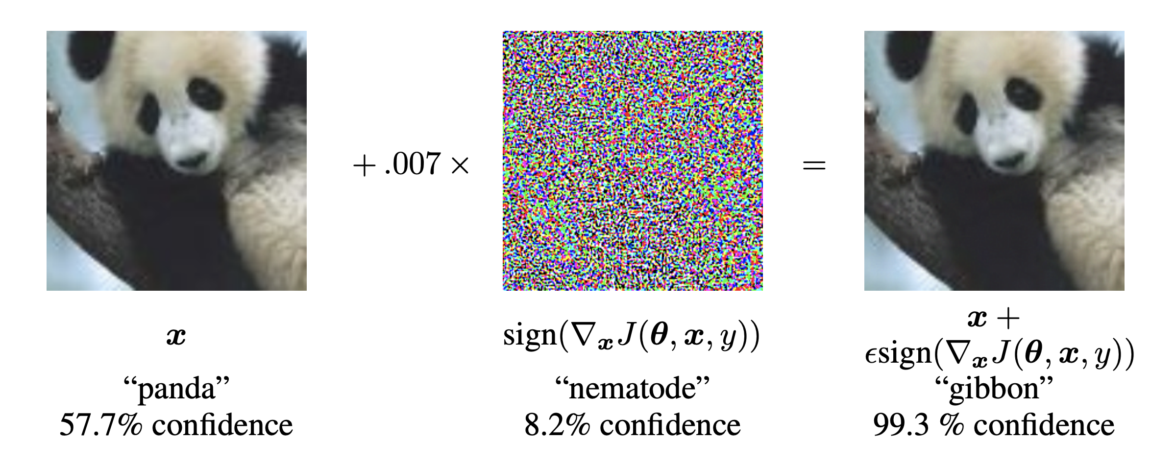
Counterfactuals … as in Adversarial Examples?
Yes and no!
While both are methodologically very similar, adversarial examples are meant to go undetected while CEs ought to be meaningful.
Desiderata
- closeness: the average distance between factual and counterfactual features should be small (Wachter, Mittelstadt, and Russell (2017))
- actionability: the proposed feature perturbation should actually be actionable (Ustun, Spangher, and Liu (2019), Poyiadzi et al. (2020))
- plausibility: the counterfactual explanation should be plausible to a human (Joshi et al. (2019))
- unambiguity: a human should have no trouble assigning a label to the counterfactual (Schut et al. (2021))
- sparsity: the counterfactual explanation should involve as few individual feature changes as possible (Schut et al. (2021))
- robustness: the counterfactual explanation should be robust to domain and model shifts (Upadhyay, Joshi, and Lakkaraju (2021))
- diversity: ideally multiple diverse counterfactual explanations should be provided (Mothilal, Sharma, and Tan (2020))
- causality: counterfactual explanations reflect the structural causal model underlying the data generating process (Karimi et al. (2020), Karimi, Schölkopf, and Valera (2021))
From Counterfactual Explanations to Algorithmic Recourse
“You cannot appeal to (algorithms). They do not listen. Nor do they bend.”
— Cathy O’Neil in Weapons of Math Destruction, 2016

Algorithmic Recourse
. . .
- O’Neil (2016) points to various real-world involving black-box models and affected individuals facing adverse outcomes.
. . .
- These individuals generally have no way to challenge their outcome.
. . .
Counterfactual Explanations that involve actionable and realistic feature perturbations can be used for the purpose of Algorithmic Recourse.
CounterfactualExplanations.jl 📦


- A unifying framework for generating Counterfactual Explanations.
- Fast, extensible and composable allowing users and developers to add and combine different counterfactual generators.
- Implements a number of SOTA generators.
- Built in Julia, but can be used to explain models built in R and Python (still experimental).
- Status 🔁: ready for research, not production. Thought/challenge/contributions welcome!

Julia has an edge with respect to Trustworthy AI: it’s open-source, uniquely transparent and interoperable 🔴🟢🟣
Probabilistic Methods for Counterfactual Explanations
When people say that counterfactuals should look realistic or plausible, they really mean that counterfactuals should be generated by the same Data Generating Process (DGP) as the factuals:
\[ x\prime \sim p(x) \]
But how do we estimate \(p(x)\)? Two probabilistic approaches …
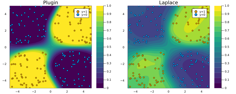
Schut et al. (2021) note that by maximizing predictive probabilities \(\sigma(M(x\prime))\) for probabilistic models \(M\in\mathcal{\widetilde{M}}\) one implicitly minimizes epistemic and aleotoric uncertainty.
\[ x\prime = \arg \min_{x\prime} \ell(M(x\prime),t) \ \ \ , \ \ \ M\in\mathcal{\widetilde{M}} \tag{7}\]

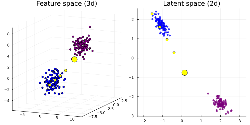
Instead of perturbing samples directly, some have proposed to instead traverse a lower-dimensional latent embedding learned through a generative model (Joshi et al. 2019).
\[ z\prime = \arg \min_{z\prime} \ell(M(dec(z\prime)),t) + \lambda h(x\prime) \tag{8}\]
and
\[x\prime = dec(z\prime)\]
where \(dec(\cdot)\) is the decoder function.
Motivation
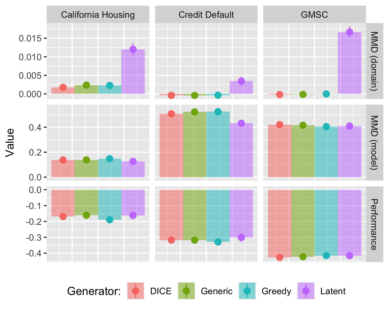
TL;DR: We find that standard implementation of various SOTA approaches to AR can induce substantial domain and model shifts. We argue that these dynamics indicate that individual recourse generates hidden external costs and provide mitigation strategies.
In this work we investigate what happens if Algorithmic Recourse is actually implemented by a large number of individuals.
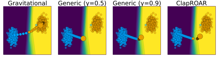
Figure 7 illustrates what we mean by Endogenous Macrodynamics in Algorithmic Recourse:
- Panel (a): we have a simple linear classifier trained for binary classification where samples from the negative class (y=0) are marked in blue and samples of the positive class (y=1) are marked in orange
- Panel (b): the implementation of AR for a random subset of individuals leads to a noticable domain shift
- Panel (c): as the classifier is retrained we observe a corresponding model shift (Upadhyay, Joshi, and Lakkaraju 2021)
- Panel (d): as this process is repeated, the decision boundary moves away from the target class.
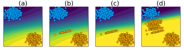
We argue that these shifts should be considered as an expected external cost of individual recourse and call for a paradigm shift from individual to collective recourse in these types of situations.
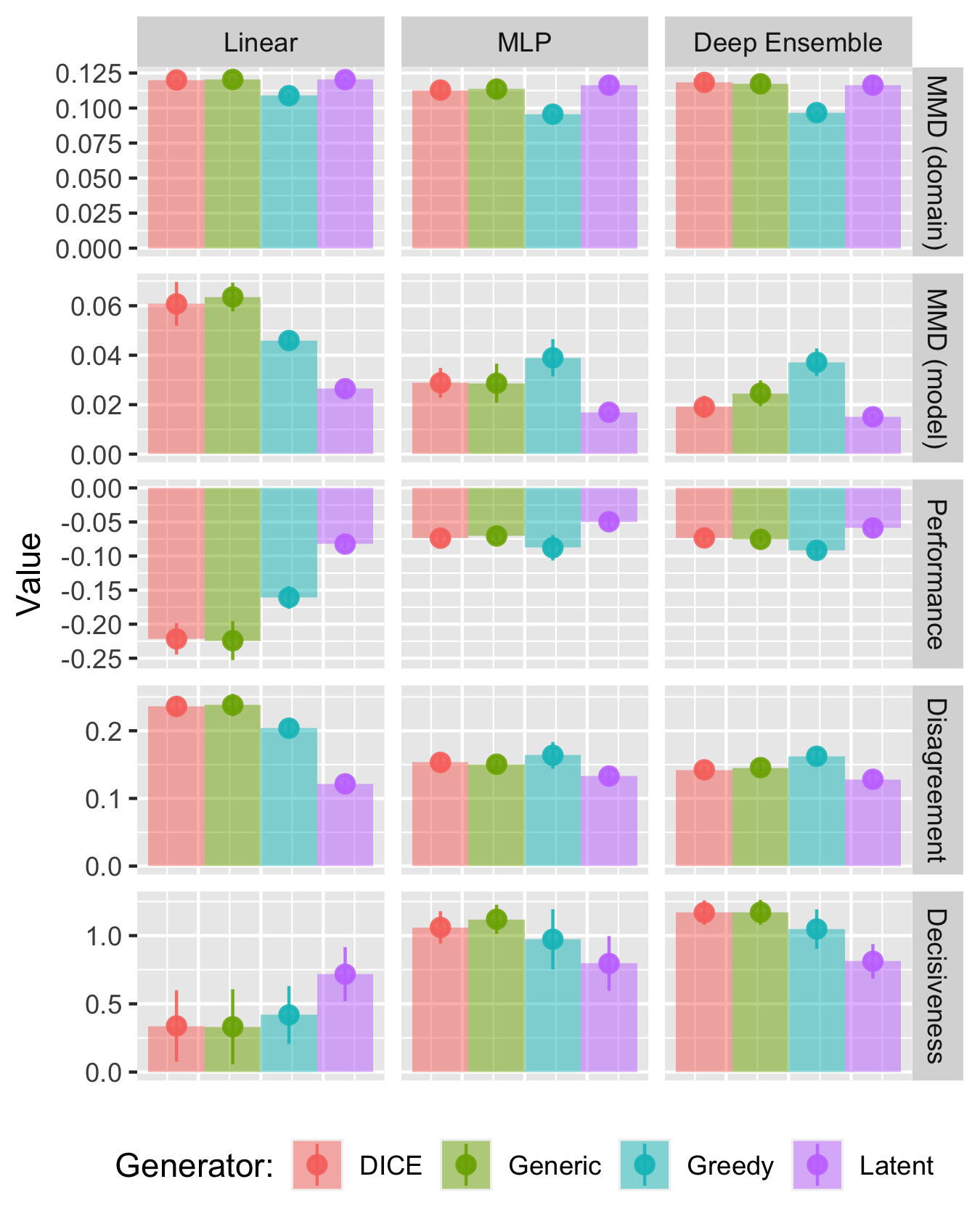
Findings
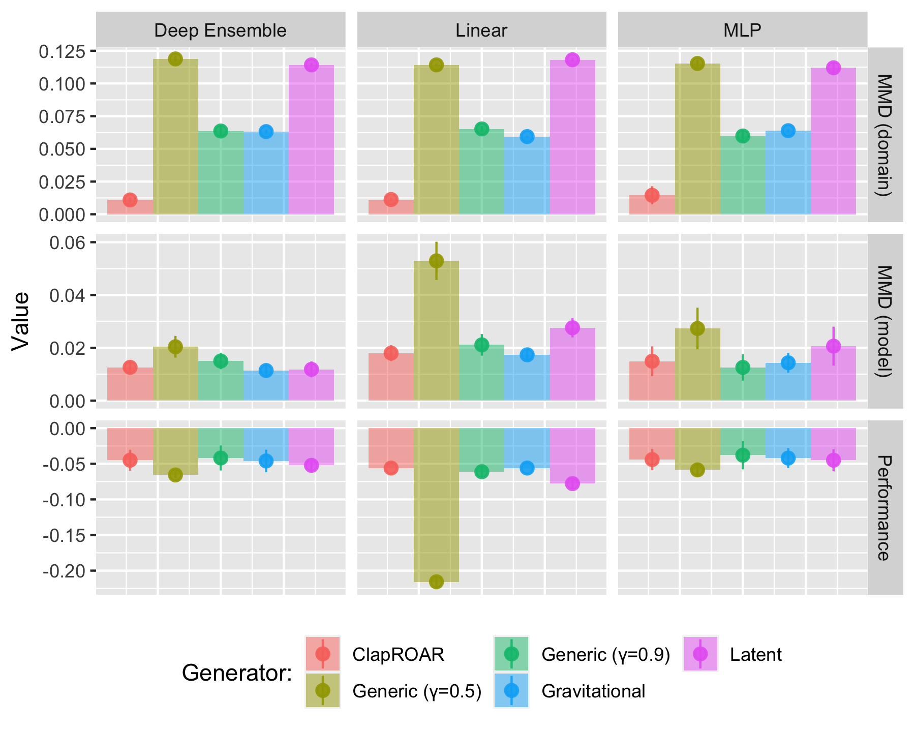
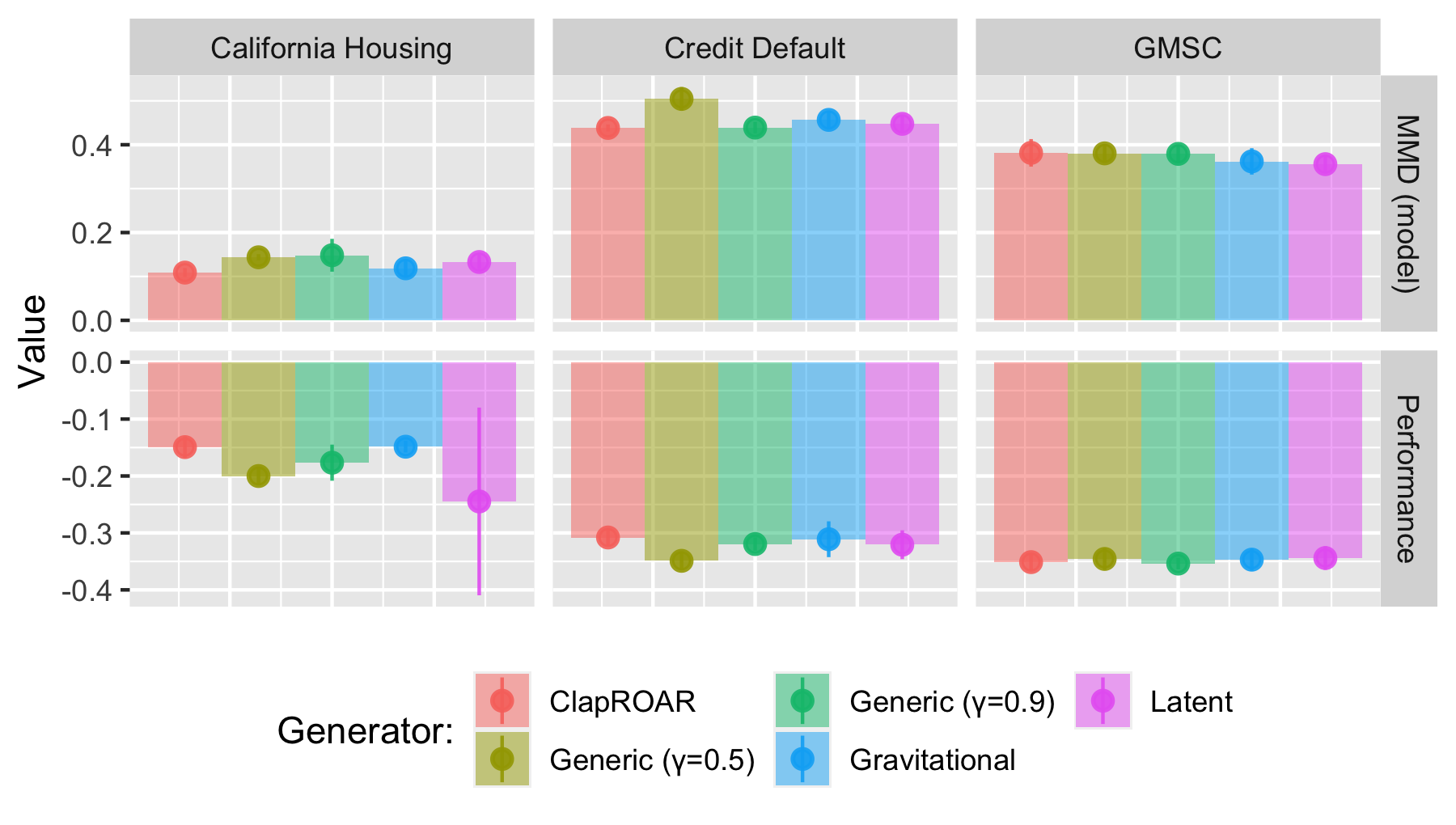
Mitigation Strategies
- Choose more conservative decision thresholds.
- Classifer Preserving ROAR (ClaPROAR): penalise classifier loss.
\[ \begin{aligned} \text{extcost}(f(\mathbf{s}^\prime)) = l(M(f(\mathbf{s}^\prime)),y^\prime) \end{aligned} \tag{11}\]
- Gravitational Counterfactual Explanations: penalise distance to some sensible point in the target domain.
\[ \begin{aligned} \text{extcost}(f(\mathbf{s}^\prime)) = \text{dist}(f(\mathbf{s}^\prime),\bar{x}) \end{aligned} \tag{12}\]
Effortless Bayesian Deep Learning through Laplace Redux

LaplaceRedux.jl (formerly BayesLaplace.jl) is a small package that can be used for effortless Bayesian Deep Learning and Logistic Regression trough Laplace Approximation. It is inspired by this Python library and its companion paper.

ConformalPrediction.jl


ConformalPrediction.jl is a package for Uncertainty Quantification (UQ) through Conformal Prediction (CP) in Julia. It is designed to work with supervised models trained in MLJ (Blaom et al. 2020). Conformal Prediction is distribution-free, easy-to-understand, easy-to-use and model-agnostic.
More Resources 📚
Read on …
- Blog post introducing CE: [TDS], [blog].
- Blog post on Laplace Redux: [TDS], [blog].
- Blog post on Conformal Prediction: [TDS], [blog].
… or get involved! 🤗
- Contributor’s Guide for
CounterfactualExplanations.jl - Contributor’s Guide for
ConformalPrediction.jl
