A year of using Quarto with Julia
Tips and tricks for Julia practitioners — Julia Eindhoven
Quick Intro
- Currently 2nd year of PhD in Trustworthy Artificial Intelligence at Delft University of Technology.
- Working on Counterfactual Explanations and Probabilistic Machine Learning with applications in Finance.
- Previously, educational background in Economics and Finance and two years at the Bank of England.
- Enthusiastic about free open-source software, in particular Julia and Quarto.


… to Quarto
- Generate multiple different output formats with ease:
- The old school: \(\LaTeX\) and PDF (including Beamer); MS Office
- The brave new world: beautiful, dynamic HTML content
- websites
- e-books
- apps
- …
- All of this starting from the same place …

A plain Markdown document blended with your favorite programming language and a YAML header defining your output.
Code chunks
Most science today involves code.
Often code forms such an integral part of the science, that it deserves its place in the final publication.
Using simple YAML options, we can specify how code is displayed. For example, we may want to use code folding to avoid unnecessary interruptions or hide large code chunks like this one that builds Figure 1.
Code
using Javis, Animations, Colors
www_path = "www/images"
_size = 600
radius_factor = 0.33
function ground(args...)
background("transparent")
sethue("white")
end
function rotate_anim(idx::Number, total::Number)
distance_circle = 0.875
steps = collect(range(distance_circle,1-distance_circle,length=total))
Animation(
[0, 1], # must go from 0 to 1
[0, steps[idx]*2π],
[sineio()],
)
end
translate_anim = Animation(
[0, 1], # must go from 0 to 1
[O, Point(_size*radius_factor, 0)],
[sineio()],
)
translate_back_anim = Animation(
[0, 1], # must go from 0 to 1
[O, Point(-(_size*radius_factor), 0)],
[sineio()],
)
julia_colours = Dict(
:blue => "#4063D8",
:green => "#389826",
:purple => "#9558b2",
:red => "#CB3C33"
)
colour_order = [:red, :purple, :green, :blue]
n_colours = length(julia_colours)
function color_anim(start_colour::String, quarto_col::String="#4b95d0")
Animation(
[0, 1], # must go from 0 to 1
[Lab(color(start_colour)), Lab(color(quarto_col))],
[sineio()],
)
end
video = Video(_size, _size)
frame_starts = 1:10:40
n_total = 250
n_frames = 150
Background(1:n_total, ground)
# Blob:
function element(; radius = 1)
circle(O, radius, :fill) # The 4 is to make the circle not so small
end
# Cross:
function cross(color="black";orientation=:horizontal)
sethue(color)
setline(10)
if orientation==:horizontal
out = line(Point(-_size,0),Point(_size,0), :stroke)
else
out = line(Point(0,-_size),Point(0,_size), :stroke)
end
return out
end
for (i, frame_start) in enumerate(1:10:40)
# Julia circles:
blob = Object(frame_start:n_total, (args...;radius=1) -> element(;radius=radius))
act!(blob, Action(1:Int(round(n_frames*0.25)), change(:radius, 1 => 75))) # scale up
act!(blob, Action(n_frames:(n_frames+50), change(:radius, 75 => 250))) # scale up further
act!(blob, Action(1:30, translate_anim, translate()))
act!(blob, Action(31:120, rotate_anim(i, n_colours), rotate_around(Point(-(_size*radius_factor), 0))))
act!(blob, Action(121:150, translate_back_anim, translate()))
act!(blob, Action(1:150, color_anim(julia_colours[colour_order[i]]), sethue()))
# Quarto cross:
cross_h = Object((n_frames+50):n_total, (args...) -> cross(;orientation=:horizontal))
cross_v = Object((n_frames+50):n_total, (args...) -> cross(;orientation=:vertical))
end
render(
video;
pathname = joinpath(www_path, "julia_quarto.gif"),
)
Javis.jl.
Dynamic Visualizations
Scientific Ideas can often be most effectively communicated through dynamic visualizations.
using Plots
using StatsBase
steps = randn(1)
T = 100
anim = @animate for t in 2:T
append!(steps, randn(1))
random_walk = cumsum(steps)
p1 = plot(random_walk, color=1, label="", title="A Gaussian random walk ...", xlims=(0,T))
acf = autocor(random_walk)
p2 = bar(acf, color=1, label="", title="... is non-stationary", xlims=(0,10), ylims=(0,1))
plot(p1, p2, size=(800,300))
end
gif(anim, fps=5)
Meeting Varying Requirements
Quarto has fantastic support for traditional and modern scholarly writing.
The challenge …
. . .
Some people still prefer to read paper or work with MS Office. Most scientific journals, for example, still work with PDF and \(\LaTeX\).

… and Quarto’s answer
. . .
Equations like Equation 1 (as well as Sections, Figures, Theorems, …) can be cross-referenced in a standardized way.
\[ \begin{aligned} Z &= \sum_{t=0}^T X_t, && X_t \sim N(\mu, \sigma) \end{aligned} \tag{1}\]
Julia Packages
Documenter.jland Quarto generally play nicely with each other (both Markdown based).
- You get some stuff for free, e.g. citation management. Unfortunately, still no support for cross-referencing …
- The use of
jldoctestis not always straight-forward (see here). Letting docs run through the Quarto engine provides an additional layer of quality assurance. - Admonitions can be used as follows (see related discussion):
As an example, we will look at … 🥁
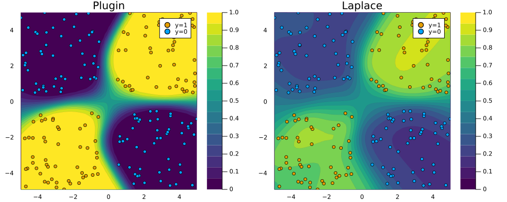
LaplaceRedux.jl


LaplaceRedux.jl is a library written in pure Julia that can be used for effortless Bayesian Deep Learning trough Laplace Approximation (LA).
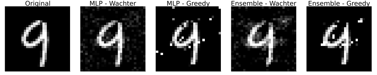
CounterfactualExplanations.jl

CounterfactualExplanations.jl is a package for generating Counterfactual Explanations (CE) and Algorithmic Recourse (AR) for black-box algorithms. Both CE and AR are related tools for explainable artificial intelligence (XAI). While the package is written purely in Julia, it can be used to explain machine learning algorithms developed and trained in other popular programming languages like Python and R. See below for short introduction and other resources or dive straight into the docs.
LaplaceRedux.jl
JuliaCon 22: Effortless Bayesian Deep Learning through Laplace Redux
LaplaceRedux.jl is a small package that can be used for effortless Bayesian Deep Learning and Logistic Regression trough Laplace Approximation. It is inspired by this Python library and its companion paper.
ConformalPrediction.jl

ConformalPrediction.jl is a package for Uncertainty Quantification (UQ) through Conformal Prediction (CP) in Julia. It is designed to work with supervised models trained in MLJ (Blaom et al. 2020). Conformal Prediction is distribution-free, easy-to-understand, easy-to-use and model-agnostic.
More Resources 📚
Read on …
- Related blog posts (hosted on this website that itself is built with Quarto and involves lots of Julia content): [1] and [2].
- Blog post introducing CE: [TDS], [blog].
- Blog post on Laplace Redux: [TDS], [blog].
- Blog post on Conformal Prediction: [TDS], [blog].
… or get involved! 🤗
- Contributor’s Guide for
CounterfactualExplanations.jl - Contributor’s Guide for
ConformalPrediction.jl
