Explaining Black-Box Models through Counterfactuals
JuliaCon 2022
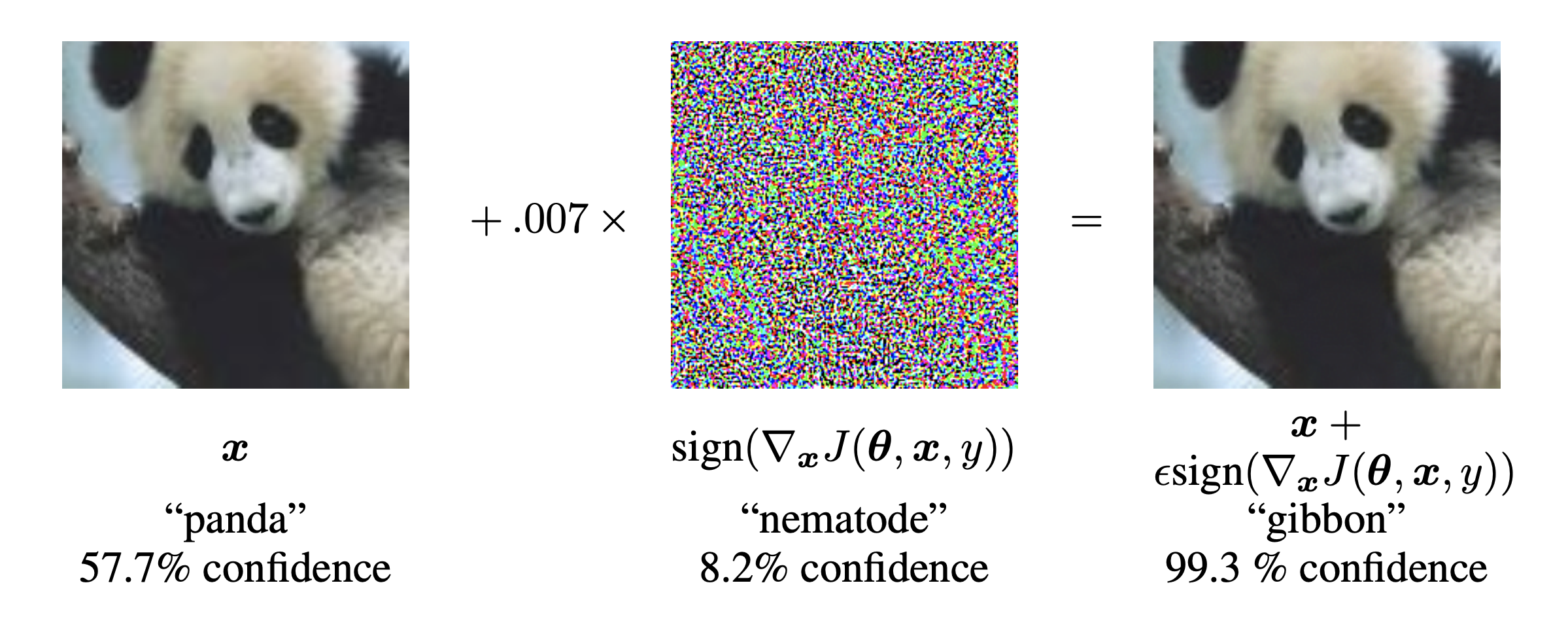
Short Lists, Pandas and Gibbons
From human to data-driven decision-making …
- Black-box models like deep neural networks are being deployed virtually everywhere.
- Includes safety-critical and public domains: health care, autonomous driving, finance, …
- More likely than not that your loan or employment application is handled by an algorithm.
… where black boxes are recipe for disaster.
- We have no idea what exactly we’re cooking up …
- Have you received an automated rejection email? Why didn’t you “mEet tHe sHoRtLisTiNg cRiTeRia”? 🙃
- … but we do know that some of it is junk.
“Weapons of Math Destruction”
“You cannot appeal to (algorithms). They do not listen. Nor do they bend.”
— Cathy O’Neil in Weapons of Math Destruction, 2016

- If left unchallenged, these properties of black-box models can create undesirable dynamics in automated decision-making systems:
- Human operators in charge of the system have to rely on it blindly.
- Individuals subject to the decisions generally have no way to challenge their outcome.
A Framework for Counterfactual Explanations
Even though […] interpretability is of great importance and should be pursued, explanations can, in principle, be offered without opening the “black box”. (Wachter et al. 2017)
Framework
. . .
Objective originally proposed by Wachter et al. (2017) is as follows
\[ \min_{x\prime \in \mathcal{X}} h(x\prime) \ \ \ \mbox{s. t.} \ \ \ M(x\prime) = t \tag{5}\]
where \(h\) relates to the complexity of the counterfactual and \(M\) denotes the classifier.
. . .
Typically this is approximated through regularization:
\[ x\prime = \arg \min_{x\prime} \ell(M(x\prime),t) + \lambda h(x\prime) \tag{6}\]
Intuition
. . .

Probabilistic Methods for Counterfactual Explanations
When people say that counterfactuals should look realistic or plausible, they really mean that counterfactuals should be generated by the same Data Generating Process (DGP) as the factuals:
\[ x\prime \sim p(x) \]
But how do we estimate \(p(x)\)? Two probabilistic approaches …
Schut et al. (2021) note that by maximizing predictive probabilities \(\sigma(M(x\prime))\) for probabilistic models \(M\in\mathcal{\widetilde{M}}\) one implicitly minimizes epistemic and aleotoric uncertainty.
\[ x\prime = \arg \min_{x\prime} \ell(M(x\prime),t) \ \ \ , \ \ \ M\in\mathcal{\widetilde{M}} \tag{7}\]

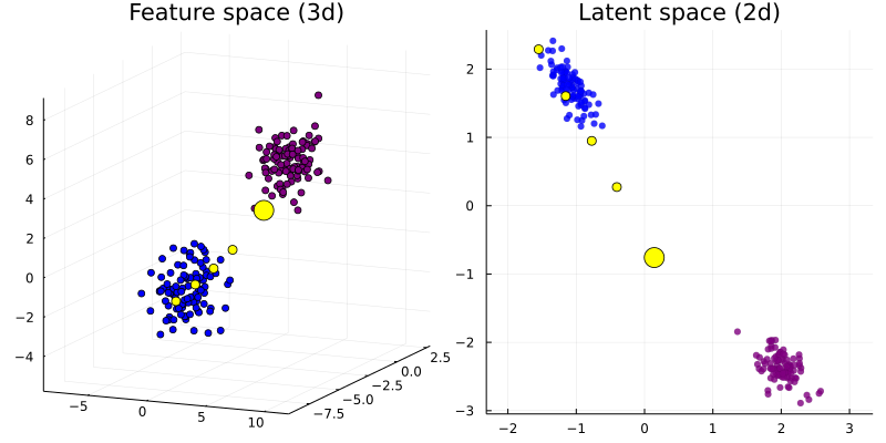
Instead of perturbing samples directly, some have proposed to instead traverse a lower-dimensional latent embedding learned through a generative model (Joshi et al. 2019).
\[ z\prime = \arg \min_{z\prime} \ell(M(dec(z\prime)),t) + \lambda h(x\prime) \tag{8}\]
and
\[x\prime = dec(z\prime)\]
where \(dec(\cdot)\) is the decoder function.
Limited Software Availability
Work currently scattered across different GitHub repositories …
- Only one unifying Python library: CARLA (Pawelczyk et al. 2021).
- Comprehensive and (somewhat) extensible.
- But not language-agnostic and some desirable functionality not supported.
- Also not composable: each generator is treated as different class/entity.
- Both R and Julia lacking any kind of implementation.

Enter: CounterfactualExplanations.jl 📦


… until now!
- A unifying framework for generating Counterfactual Explanations.
- Built in Julia, but essentially language agnostic:
- Currently supporting explanations for differentiable models built in Julia (e.g. Flux) and torch (R and Python).
- Designed to be easily extensible through dispatch.
- Designed to be composable allowing users and developers to combine different counterfactual generators.

Julia has an edge with respect to Trustworthy AI: it’s open-source, uniquely transparent and interoperable 🔴🟢🟣
Overview
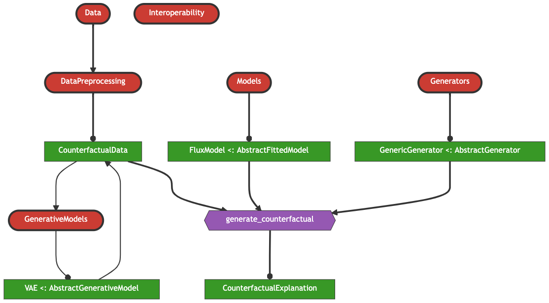
Generators
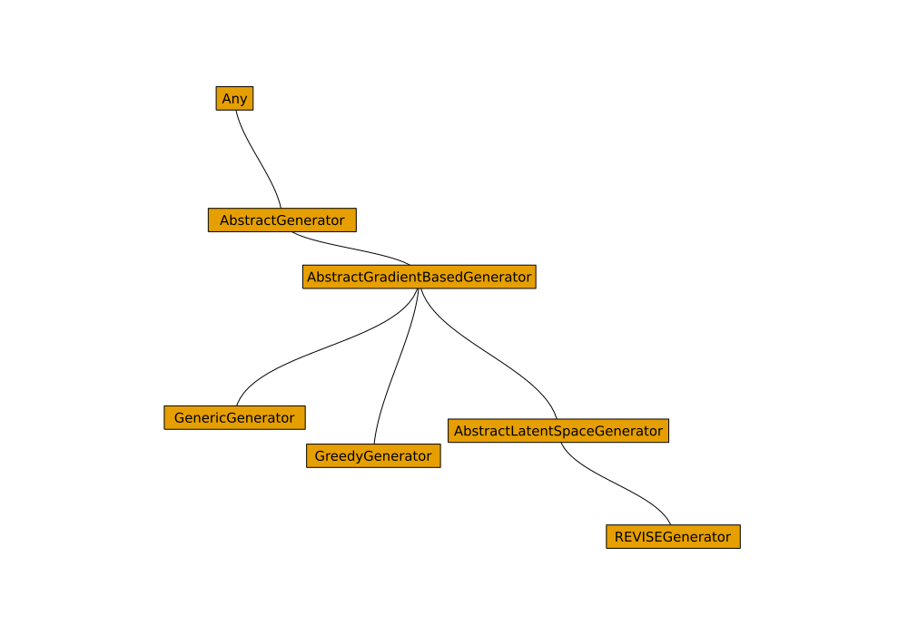
AbstractGenerator.
Models
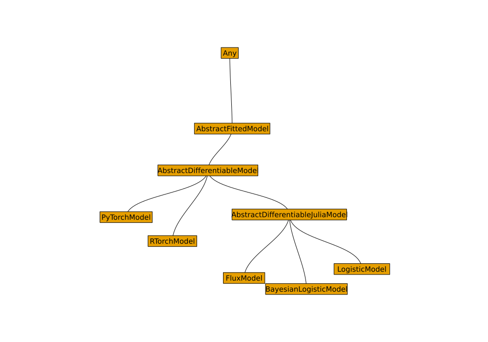
AbstractFittedModel.
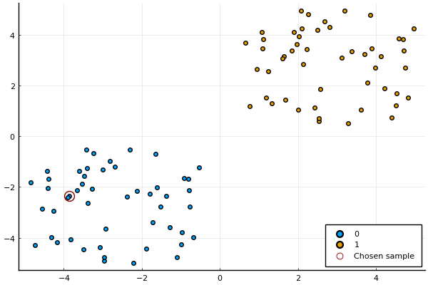
A simple example
- Load and prepare some toy data.
- Select a random sample.
- Generate counterfactuals using different approaches.
Generic Generator
Code
. . .
We begin by instantiating the fitted model …
. . .
… then based on its prediction for \(x\) we choose the opposite label as our target …
. . .
… and finally generate the counterfactual.
Output
. . .
… et voilà!
GenericGenerator. The contour (left) shows the predicted probabilities of the classifier (Logistic Regression).
Greedy Generator
Code
. . .
This time we use a Bayesian classifier …
. . .
… and once again choose our target label as before …
. . .
… to then finally use greedy search to find a counterfactual.
Output
. . .
In this case the Bayesian approach yields a similar outcome.

GreedyGenerator. The contour (left) shows the predicted probabilities of the classifier (Bayesian Logistic Regression).
REVISE Generator
Code
Using the same classifier as before we can either use the specific REVISEGenerator …
. . .
… or realize that that REVISE (Joshi et al. 2019) just boils down to generic search in a latent space:
Output
. . .
We have essentially combined latent search with a probabilistic classifier (as in Antorán et al. (2020)).
REVISEGenerator.
MNIST - Latent Space Search
Good VAE
. . .
Loading pre-trained classifiers and VAE …
. . .
… instantiating model and attaching VAE.
. . .
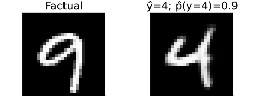
The results in Figure 13 look great!
Bad VAE
. . .
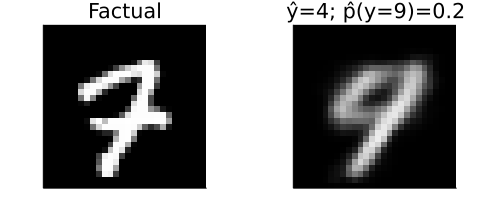
But things can also go wrong …
The VAE used to generate the counterfactual in Figure 14 is not expressive enough.
. . .
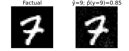
The counterfactual in Figure 15 is also valid … what to do?
Custom Models - Deep Ensemble
Step 1: add composite type as subtype of AbstractFittedModel.
Step 2: dispatch logits and probs methods for new model type.
using Statistics
import CounterfactualExplanations.Models: logits, probs
logits(M::FittedEnsemble, X::AbstractArray) = mean(Flux.stack([nn(X) for nn in M.ensemble],3), dims=3)
probs(M::FittedEnsemble, X::AbstractArray) = mean(Flux.stack([softmax(nn(X)) for nn in M.ensemble],3),dims=3)
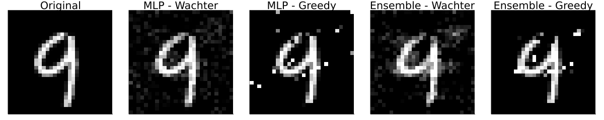
M = FittedEnsemble(ensemble)Results for a simple deep ensemble also look convincing!
Custom Models - Interoperability
Adding support for torch models was easy! Here’s how I implemented it for torch classifiers trained in R.
Source code
. . .
Step 1: add composite type as subtype of AbstractFittedModel
Implemented here.
Step 2: dispatch logits and probs methods for new model type.
Implemented here.
. . .
Step 3: add gradient access.
Implemented here.
Unchanged API
. . .

GenericGenerator and RTorchModel.
Custom Generators
Idea 💡: let’s implement a generic generator with dropout!
Dispatch
. . .
Step 1: create a subtype of AbstractGradientBasedGenerator (adhering to some basic rules).
# Constructor:
abstract type AbstractDropoutGenerator <: AbstractGradientBasedGenerator end
struct DropoutGenerator <: AbstractDropoutGenerator
loss::Symbol # loss function
complexity::Function # complexity function
mutability::Union{Nothing,Vector{Symbol}} # mutibility constraints
λ::AbstractFloat # strength of penalty
ϵ::AbstractFloat # step size
τ::AbstractFloat # tolerance for convergence
p_dropout::AbstractFloat # dropout rate
end. . .
Step 2: implement logic for generating perturbations.
import CounterfactualExplanations.Generators: generate_perturbations, ∇
using StatsBase
function generate_perturbations(generator::AbstractDropoutGenerator, counterfactual_state::State)
𝐠ₜ = ∇(generator, counterfactual_state.M, counterfactual_state) # gradient
# Dropout:
set_to_zero = sample(1:length(𝐠ₜ),Int(round(generator.p_dropout*length(𝐠ₜ))),replace=false)
𝐠ₜ[set_to_zero] .= 0
Δx′ = - (generator.ϵ .* 𝐠ₜ) # gradient step
return Δx′
endUnchanged API
. . .
DropoutGenerator and RTorchModel.
JuliaCon 2022 and beyond
To JuliaCon …
Develop package, register and submit to JuliaCon 2022.
Native support for deep learning models (Flux, torch).
Add latent space search.
… and beyond
. . .
- Add more generators:
- DiCE (Mothilal et al. 2020)
- ROAR (Upadhyay et al. 2021)
- MINT (Karimi et al. 2021)
. . .
- Add support for more models:
MLJ,GLM, …- Non-differentiable
. . .
- Enhance preprocessing functionality.
. . .
- Extend functionality to regression problems.
. . .
- Use
Fluxoptimizers.
. . .
- …