Effortless Bayesian Deep Learning through Laplace Redux
JuliaCon 2022
Enter: Bayesian Deep Learning 🔮
Yes, we can!
Popular approaches include …
MCMC (see Turing)
Variational Inference (Blundell et al. 2015)
Monte Carlo Dropout (Gal and Ghahramani 2016)
Deep Ensembles (Lakshminarayanan et al. 2017)
. . .

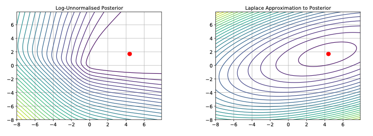
Laplace Approximation
We first need to estimate the weight posterior \(p(\theta|\mathcal{D})\) …
Idea 💡: Taylor approximation at the mode.
- Going through the maths we find that this yields a Gaussian posteriour centered around the MAP estimate \(\hat\theta\) (see pp. 148/149 in Murphy (2022)).
- Covariance corresponds to inverse Hessian at the mode (in practice we may have to rely on approximations).
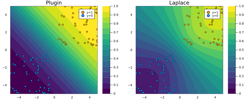
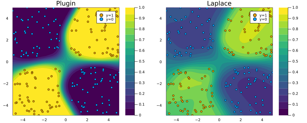
Now we can rely on MC or Probit Approximation to compute posterior predictive (classification).
LaplaceRedux.jl - a small package 📦


What started out as my first coding project Julia …
- Big fan of learning by coding so after reading the first chapters of Murphy (2022) I decided to code up Bayesian Logisitic Regression from scratch.
- I also wanted to learn Julia at the time, so tried to hit two birds with one stone.
- Outcome: 1. This blog post. 2. I have since been hooked on Julia.
… has turned into a small package 📦 with great potential.
- When coming across the NeurIPS 2021 paper on Laplace Redux for deep learning (Daxberger et al. 2021), I figured I could step it up a notch.
- Outcome:
LaplaceRedux.jland another blog post.
From Bayesian Logistic Regression …
From maths …
. . .
We assume a Gaussian prior for our weights … \[ p(\theta) \sim \mathcal{N} \left( \theta | \mathbf{0}, \lambda^{-1} \mathbf{I} \right)=\mathcal{N} \left( \theta | \mathbf{0}, \mathbf{H}_0^{-1} \right) \tag{3}\]
. . .
… which corresponds to logit binary crossentropy loss with weight decay:
\[ \ell(\theta)= - \sum_{n}^N [y_n \log \mu_n + (1-y_n)\log (1-\mu_n)] + \\ \frac{1}{2} (\theta-\theta_0)^T\mathbf{H}_0(\theta-\theta_0) \tag{4}\]
. . .
For Logistic Regression we have the Hessian in closed form (p. 338 in Murphy (2022)):
\[ \nabla_{\theta}\nabla_{\theta}^\mathsf{T}\ell(\theta) = \frac{1}{N} \sum_{n}^N(\mu_n(1-\mu_n)\mathbf{x}_n)\mathbf{x}_n^\mathsf{T} + \mathbf{H}_0 \tag{5}\]
… to code
. . .
Gotta love Julia ❤️💜💚
. . .
Logistic Regression can be done in Flux …
. . .
… but now we autograd! Leveraged in LaplaceRedux.
… to Bayesian Neural Networks
Code
. . .
An actual MLP …
. . .
… same API call:
. . .
Results
. . .
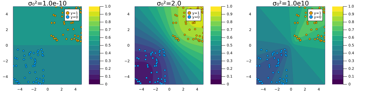
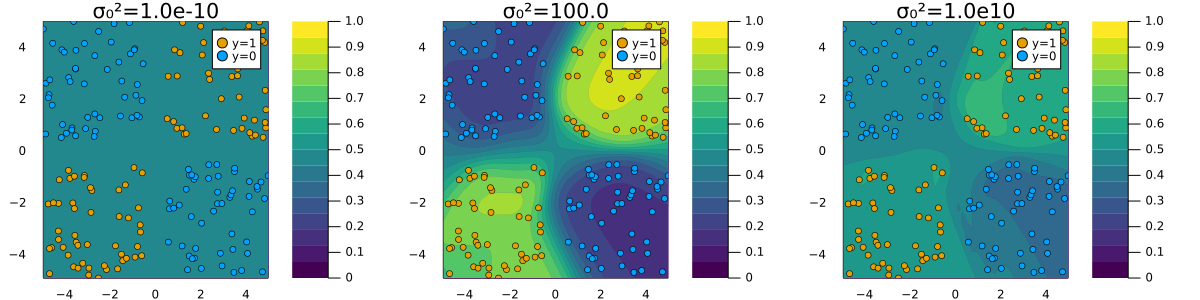
A quick note on the prior
Low prior uncertainty \(\rightarrow\) posterior dominated by prior. High prior uncertainty \(\rightarrow\) posterior approaches MLE.
Logistic Regression
MLP
A crucial detail I skipped
We’re really been using linearized neural networks …
MC fails
- Could do Monte Carlo for true BNN predictive, but this performs poorly when using approximations for the Hessian.
- Instead we rely on linear expansion of predictive around mode (Immer et al. 2020).
- Intuition: Hessian approximation involves linearization, then so should the predictive.
. . .
Applying the GNN approximation […] turns the underlying probabilistic model locally from a BNN into a GLM […] Because we have effectively done inference in the GGN-linearized model, we should instead predict using these modified features. — Immer et al. (2020)
JuliaCon 2022 and beyond
To JuliaCon …
Learn about Laplace Redux by implementing it in Julia.
Turn code into a small package.
Submit to JuliaCon 2022 and share the idea.
… and beyond
. . .
Package is bare-bones at this point and needs a lot of work.
- Goal: reach same level of maturity as Python counterpart. (Beautiful work btw!)
- Problem: limited capacity and fairly new to Julia.
- Solution: find contributors 🤗.

Specific Goals
Easy
- Still missing support for multi-class and regression.
- Due diligence: peer review and unit testing.
Harder
- Hessian approximations still quadratically large: use factorizations.
- Hyperparameter tuning: what about that prior?
- Scaling things up: subnetwork inference.
- Early stopping: do we really end up at the mode?
- …