Chapter 3 Optimization

3.1 Line search

3.1.1 Methodology

The goal of Exercise 3.1 in Nocedal and Wright (2006) is to minimize the bivariate Rosenbrock function (Equation (3.1)) using steepest descent and Newton’s method. The Rosenbrock function - also known as Rosenbrock’s banana function - has a long, narrow, parabolic shaped flat valley and is often used for to test optimization algorithms for their performance (see here).

\[ \begin{equation} f(\mathbb{x})=100(x_2-x_1^2)^2+(1-x_1)^2 \tag{3.1} \end{equation} \] We can implement Equation (3.1) in R as follows:

# Rosenbrock:
f = function(X) {
  100 * (X[2] - X[1]^2)^2 + (1 - X[1])^2
}

Figure 3.1 shows the output of the function over \(x_1,x_2 \in [-1.5, 1.5]\) along with its minimum indicated as a red asterisk and the two starting points: (1) \(X_0=(1.2,1.2)\) and (2) \(X_0=(-1.2,1)\).

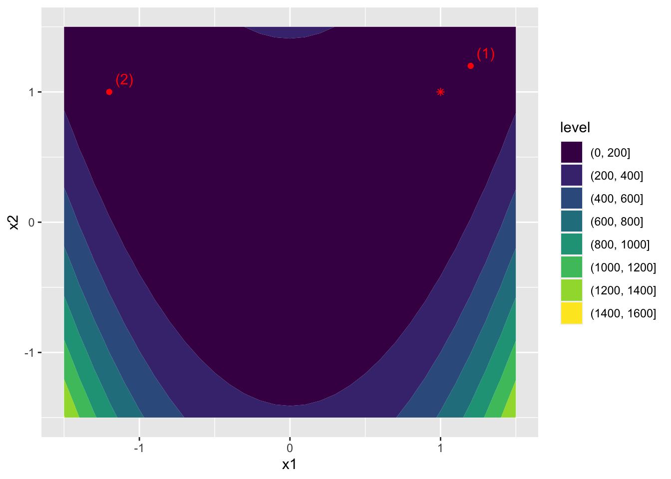
Figure 3.1: Output of the Rosenbrock function and minimizer in red.

The gradient and Hessian of \(f\) can be computed as

\[ \begin{equation} \nabla f(\mathbb{x})= \begin{pmatrix} \frac{ \partial f}{\partial x_1} \\ \frac{ \partial f}{\partial x_2} \end{pmatrix} \tag{3.2} \end{equation} \]

and

\[ \begin{equation} \nabla^2 f(\mathbb{x})= \begin{pmatrix} \frac{ \partial^2 f}{\partial x_1^2} & \frac{ \partial^2 f}{\partial x_1 \partial x_2} \\ \frac{ \partial^2 f}{\partial x_2\partial x_1} & \frac{ \partial^2 f}{\partial x_2^2} \end{pmatrix} \tag{3.3} \end{equation} \]

which in R can be encoded as follows:

# Gradient:
df = function(X) {
  df = rep(0, length(X))
  df[1] = -400 * X[1]^2 * (X[2] - X[1]^2) - 2 * (1 - X[1]) # partial with respect to x_1
  df[2] = 200 * (X[2] - X[1]^2)
  return(df)
}

# Hessian:
ddf = function(X) {
  ddf = matrix(nrow = length(X), ncol=length(X))
  ddf[1,1] = 1200 * X[1]^2 - 400 * X[2] + 2 # partial with respect to x_1
  ddf[2,1] = ddf[1,2] = -400 * X[1]
  ddf[2,2] = 200
  return(ddf)
}

For both methods I will use the Arminjo condition with backtracking. The gradient_desc function (below) can implement both steepest descent and Newton’s method. The code for the function can be inspected below. There’s also a small description of the different arguments.

function (f, df, X0, step_size0 = 1, ddf = NULL, method = "newton", c = 1e-04, remember = TRUE, tau = 1e-05, backtrack_cond = "arminjo", max_iter = 10000) 
{
    X_latest = matrix(X0)
    if (remember) {
        X = matrix(X0, ncol = length(X0))
        steps = matrix(ncol = length(X0))
    }
    iter = 0
    if (method == "steepest") {
        B = function(X) {
            diag(length(X))
        }
    }
    else if (method == "newton") {
        B = tryCatch(ddf, error = function(e) {
            stop("Hessian needs to be supplied for Newton's method.")
        })
    }
    if (backtrack_cond == "arminjo") {
        sufficient_decrease = function(alpha) {
            return(f(X_k + alpha * p_k) <= f(X_k) + c * alpha * t(df_k) %*% p_k)
        }
    }
    else if (is.na(backtrack_cond)) {
        sufficient_decrease = function(alpha) {
            return(f(X_k + alpha * p_k) <= f(X_k))
        }
    }
    while (any(abs(df(X_latest) - rep(0, length(X_latest))) > tau) & iter < max_iter) {
        X_k = X_latest
        alpha = step_size0
        df_k = matrix(df(X_latest))
        B_k = B(X_latest)
        p_k = qr.solve(-B_k, df_k)
        while (!sufficient_decrease(alpha)) {
            alpha = alpha/2
        }
        X_latest = X_latest + alpha * p_k
        iter = iter + 1
        if (remember) {
            X = rbind(X, t(X_latest))
            steps = rbind(steps, t(alpha * p_k))
        }
    }
    if (iter >= max_iter) 
        warning("Reached maximum number of iterations without convergence.")
    output = list(optimal = X_latest, visited = tryCatch(X, error = function(e) NULL), steps = tryCatch(steps, error = function(e) NULL), X0 = X0, method = method)
    return(output)
}

Similarly you can take a look at how the gradient_desc is applied in the underlying problem by unhiding the next code chunk.

library(fromScratchR)
init_guesses = 1:nrow(X0)
algos = c("steepest","newton")
grid = expand.grid(guess=init_guesses,algo=algos)
X_star = lapply(
  1:nrow(grid),
  function(i) {
    gradient_desc(
      f=f,df=df,
      X0=X0[grid[i,"guess"],c(x1,x2)],
      method = grid[i,"algo"]
    )
  }
)
# Tidy up
X_star_dt = rbindlist(
  lapply(
    1:length(X_star), 
    function(i) {
      dt = data.table(X_star[[i]]$visited)
      dt[,method:=X_star[[i]]$method]
      dt[,(c("x0_1","x0_2")):=.(X_star[[i]]$X0[1],X_star[[i]]$X0[2])]
      dt[,iteration:=.I-1]
      dt[,y:=f(c(V1,V2)),by=.(1:nrow(dt))]
    }
  )
)

3.1.2 Results

The below shows how the two algorithms converge to

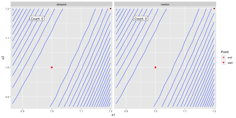
Figure 3.2: Good initial guess.

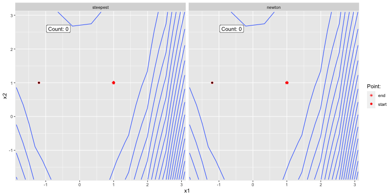
Figure 3.3: Poor initial guess.