Explaining Black-Box Models through Counterfactuals

Authors

Affiliation

Patrick Altmeyer

Delft University of Technology

Arie van Deursen

Delft University of Technology

Cynthia C. S. Liem

Delft University of Technology

Abstract

We present CounterfactualExplanations.jl: a package for generating Counterfactual Explanations (CE) and Algorithmic Recourse (AR) for black-box models in Julia. CE explain how inputs into a model need to change to yield specific model predictions. Explanations that involve realistic and actionable changes can be used to provide AR: a set of proposed actions for individuals to change an undesirable outcome for the better. In this article, we discuss the usefulness of CE for Explainable Artificial Intelligence and demonstrate the functionality of our package. The package is straightforward to use and designed with a focus on customization and extensibility. We envision it to one day be the go-to place for explaining arbitrary predictive models in Julia through a diverse suite of counterfactual generators.

Keywords

Julia, Explainable Artificial Intelligence, Counterfactual Explanations, Algorithmic Recourse

1 Introduction

Machine Learning models like Deep Neural Networks have become so complex and opaque over recent years that they are generally considered black-box systems. This lack of transparency exacerbates several other problems typically associated with these models: they tend to be unstable (Goodfellow, Shlens, and Szegedy 2014), encode existing biases (Buolamwini and Gebru 2018) and learn representations that are surprising or even counter-intuitive from a human perspective (Buolamwini and Gebru 2018). Nonetheless, they often form the basis for data-driven decision-making systems in real-world applications.

As others have pointed out, this scenario gives rise to an undesirable principal-agent problem involving a group of principals—i.e. human stakeholders—that fail to understand the behaviour of their agent—i.e. the black-box system (Borch 2022). The group of principals may include programmers, product managers and other decision-makers who develop and operate the system as well as those individuals ultimately subject to the decisions made by the system. In practice, decisions made by black-box systems are typically left unchallenged since the group of principals cannot scrutinize them:

“You cannot appeal to (algorithms). They do not listen. Nor do they bend.” (O’Neil 2016)

In light of all this, a quickly growing body of literature on Explainable Artificial Intelligence (XAI) has emerged. Counterfactual Explanations fall into this broad category. They can help human stakeholders make sense of the systems they develop, use or endure: they explain how inputs into a system need to change for it to produce different decisions. Explainability benefits internal as well as external quality assurance. Explanations that involve plausible and actionable changes can be used for Algorithmic Recourse (AR): they offer the group of principals a way to not only understand their agent’s behaviour but also adjust or react to it.

The availability of open-source software to explain black-box models through counterfactuals is still limited. Through the work presented here, we aim to close that gap and thereby contribute to broader community efforts towards XAI. We envision this package to one day be the go-to place for Counterfactual Explanations in Julia. Thanks to Julia’s unique support for interoperability with foreign programming languages we believe that this library may also benefit the broader machine learning and data science community.

Our package provides a simple and intuitive interface to generate CE for many standard classification models trained in Julia, as well as in Python and R. It comes with detailed documentation involving various illustrative example datasets, models and counterfactual generators for binary and multi-class prediction tasks. A carefully designed package architecture allows for a seamless extension of the package functionality through custom generators and models.

The remainder of this article is structured as follows: Section 2 presents related work on XAI as well as a brief overview of the methodological framework underlying CE. Section 3 introduces the Julia package and its high-level architecture. Section 4 presents several basic and advanced usage examples. In Section 5 we demonstrate how the package functionality can be customized and extended. To illustrate its practical usability, we explore examples involving real-world data in Section 6. Finally, we also discuss the current limitations of our package, as well as its future outlook in Section 7. Section 8 concludes.

2 Background and related work

In this section, we first briefly introduce the broad field of Explainable AI, before narrowing it down to Counterfactual Explanations. We introduce the methodological framework and finally point to existing open-source software.

2.1 Literature on Explainable AI

The field of XAI is still relatively young and made up of a variety of subdomains, definitions, concepts and taxonomies. Covering all of these is beyond the scope of this article, so we will focus only on high-level concepts. The following literature surveys provide more detail: Arrieta et al. (2020) provide a broad overview of XAI (Arrieta et al. 2020); Fan et al. (2020) focus on explainability in the context of deep learning (Fan, Xiong, and Wang 2020); and finally, Karimi et al. (2020) (Karimi, Barthe, et al. 2020) and Verma et al. (2020) Verma, Dickerson, and Hines (2020) offer detailed reviews of the literature on Counterfactual Explanations and Algorithmic Recourse (see also Molnar (2020) and Varshney (2022)). Miller (2019) explicitly discusses the concept of explainability from the perspective of a social scientist (Miller 2019).

The first broad distinction we want to make here is between Interpretable and Explainable AI. These terms are often used interchangeably, but this can lead to confusion. We find the distinction made in Rudin (2019) useful: Interpretable AI involves models that are inherently interpretable and transparent such as general additive models (GAM), decision trees and rule-based models; Explainable AI involves models that are not inherently interpretable but require additional tools to be explainable to humans. Examples of the latter include Ensembles, Support Vector Machines and Deep Neural Networks. Some would argue that we best avoid the second category of models altogether and instead focus solely on interpretable AI Rudin (2019). While we agree that initial efforts should always be geared towards interpretable models, avoiding black boxes altogether would entail missed opportunities and anyway is probably not very realistic at this point. For that reason, we expect the need for XAI to persist in the medium term. Explainable AI can further be broadly divided into global and local explainability: the former is concerned with explaining the average behaviour of a model, while the latter involves explanations for individual predictions (Molnar 2020). Tools for global explainability include partial dependence plots (PDP), which involve the computation of marginal effects through Monte Carlo, and global surrogates. A surrogate model is an interpretable model that is trained to explain the predictions of a black-box model.

Counterfactual Explanations fall into the category of local methods: they explain how individual predictions change in response to individual feature perturbations. Among the most popular alternatives to Counterfactual Explanations are local surrogate explainers including Local Interpretable Model-agnostic Explanations (LIME) and Shapley additive explanations (SHAP). Since explanations produced by LIME and SHAP typically involve simple feature importance plots, they arguably rely on reasonably interpretable features at the very least. Contrary to Counterfactual Explanations, for example, it is not obvious how to apply LIME and SHAP to high-dimensional image data. Nonetheless, local surrogate explainers are among the most widely used XAI tools today, potentially because they are easy to interpret and implemented in popular programming languages. Proponents of surrogate explainers also commonly mention that there is a straightforward way to assess their reliability: a surrogate model that generates predictions in line with those produced by the black-box model is said to have high fidelity and therefore considered reliable. As intuitive as this notion may be, it also points to an obvious shortfall of surrogate explainers: even a high-fidelity surrogate model that produces the same predictions as the black-box model 99 per cent of the time is useless and potentially misleading for every 1 out of 100 individual predictions.

A recent study has shown that even experienced data scientists tend to put too much trust in explanations produced by LIME and SHAP (Kaur et al. 2020). Another recent work has shown that both methods can be easily fooled: they depend on random input perturbations, a property that can be abused by adverse agents to essentially whitewash strongly biased black-box models (Slack et al. 2020). In related work, the same authors find that while gradient-based Counterfactual Explanations can also be manipulated, there is a straightforward way to protect against this in practice (Slack et al. 2021). In the context of quality assessment, it is also worth noting that—contrary to surrogate explainers—CE always achieve full fidelity by construction: counterfactuals are searched with respect to the black-box classifier, not some proxy for it. That being said, CE should also be used with care and research around them is still in its early stages.

2.2 A framework for Counterfactual Explanations

Counterfactual search involves feature perturbations: we are interested in understanding how we need to change individual attributes in order to change the model output to a desired value or label (Molnar 2020). Typically the underlying methodology is presented in the context of binary classification: \(M: \mathcal{X} \mapsto \mathcal{Y}\) where \(\mathcal{X}\subset\mathbb{R}^D\) and \(\mathcal{Y}=\{0,1\}\). Further, let \(t=1\) be the target class and let \(x\) denote the factual feature vector of some individual sample outside of the target class, so \(y=M(x)=0\). We follow this convention here, though it should be noted that the ideas presented here also carry over to multi-class problems and regression (Molnar 2020).

The counterfactual search objective originally proposed by Wachter, Mittelstadt, and Russell (2017) is as follows

\[ \min_{x^\prime \in \mathcal{X}} h(x^\prime) \ \ \ \mbox{s. t.} \ \ \ M(x^\prime) = t \tag{1}\]

where \(h(\cdot)\) quantifies how complex or costly it is to go from the factual \(x\) to the counterfactual \(x^\prime\). To simplify things we can restate this constrained objective as the following unconstrained and differentiable problem:

\[ x^\prime = \arg \min_{x^\prime} \ell(M(x^\prime),t) + \lambda h(x^\prime) \tag{2}\]

Here \(\ell\) denotes some loss function targeting the deviation between the target label and the predicted label and \(\lambda\) governs the strength of the complexity penalty. Provided we have gradient access for the black-box model \(M\) the solution to this problem can be found through gradient descent. This generic framework lays the foundation for most state-of-the-art approaches to counterfactual search and is also used as the baseline approach in our package. The hyperparameter \(\lambda\) is typically tuned through grid search or in some sense pre-determined by the nature of the problem. Conventional choices for \(\ell\) include margin-based losses like cross-entropy loss and hinge loss. It is worth pointing out that the loss function is typically computed with respect to logits rather than predicted probabilities, a convention that we have chosen to follow.¹

Numerous extensions to this simple approach have been developed since CE were first proposed in 2017 (see Verma, Dickerson, and Hines (2020) and Karimi, Barthe, et al. (2020) for surveys). The various approaches largely differ in that they use different flavours of search objective defined in Equation 2. Different penalties are often used to address many of the desirable properties of effective CE that have been set out. These desiderata include: proximity — the distance between factual and counterfactual features should be small (Wachter, Mittelstadt, and Russell 2017); actionability — the proposed recourse should be actionable (Ustun, Spangher, and Liu 2019; Poyiadzi et al. 2020); plausibility — the counterfactual explanation should be plausible to a human (Joshi et al. 2019; Schut et al. 2021); sparsity — the counterfactual explanation should involve as few individual feature changes as possible (Schut et al. 2021); robustness — the counterfactual explanation should be robust to domain and model shifts (Upadhyay, Joshi, and Lakkaraju 2021); diversity — ideally multiple diverse counterfactuals should be provided (Mothilal, Sharma, and Tan 2020); and causality — counterfactuals should respect the structural causal model underlying the data generating process (Karimi, Von Kügelgen, et al. 2020; Karimi, Schölkopf, and Valera 2021).

Beyond gradient-based counterfactual search, which has been the main focus in our development so far, various methodologies have been proposed that can handle non-differentiable models like decision trees. We have implemented some of these approaches and will discuss them further in Section 3.2.

2.3 Existing software

To the best of our knowledge, the package introduced here provides the first implementation of Counterfactual Explanations in Julia and therefore represents a novel contribution to the community. As for other programming languages, we are only aware of one other unifying framework: the Python library CARLA (Pawelczyk et al. 2021).² In addition to that, there exists open-source code for some specific approaches to CE that have been proposed in recent years. The approach-specific implementations that we have been able to find are generally well-documented, but exclusively in Python. For example, a PyTorch implementation of a greedy generator for Bayesian models proposed in Schut et al. (2021) has been released. As another example, the popular InterpretML library includes an implementation of a diverse counterfactual generator (Mothilal, Sharma, and Tan 2020).

Generally speaking, software development in the space of XAI has largely focused on various global methods and surrogate explainers: implementations of PDP, LIME and SHAP are available for both Python (e.g. lime, shap) and R (e.g. lime, iml, shapper, fastshap). In the Julia space, there exist two packages related to XAI: firstly, ShapML.jl, which provides a fast implementation of SHAP; and, secondly, ExplainableAI.jl, which enables users to easily visualise gradients and activation maps for Flux.jl models. We also should not fail to mention the comprehensive Interpretable AI infrastructure, which focuses exclusively on interpretable models.

Arguably the current availability of tools for explaining black-box models in Julia is limited, but it appears that the community is invested in changing that. The team behind MLJ.jl, for example, recruited contributors for a project about both Interpretable and Explainable AI in 2022.³ With our work on Counterfactual Explanations we hope to contribute to these efforts. We think that because of its unique transparency the Julia language naturally lends itself towards building Trustworthy AI systems.

3 Introducing: CounterfactualExplanations.jl

Figure 1 provides an overview of the package architecture. It is built around two core modules that are designed to be as extensible as possible through dispatch: 1) Models is concerned with making any arbitrary model compatible with the package; 2) Generators is used to implement counterfactual search algorithms. The core function of the package—generate_counterfactual—uses an instance of type <:AbstractFittedModel produced by the Models module and an instance of type <:AbstractGenerator produced by the Generators module. Relating this to the methodology outlined in Section 2.2, the former instance corresponds to the model \(M\), while the latter defines the rules for the counterfactual search (Equation 2).

Figure 1: High-level schematic overview of package architecture. Modules are shown in red, structs in green and functions in purple.

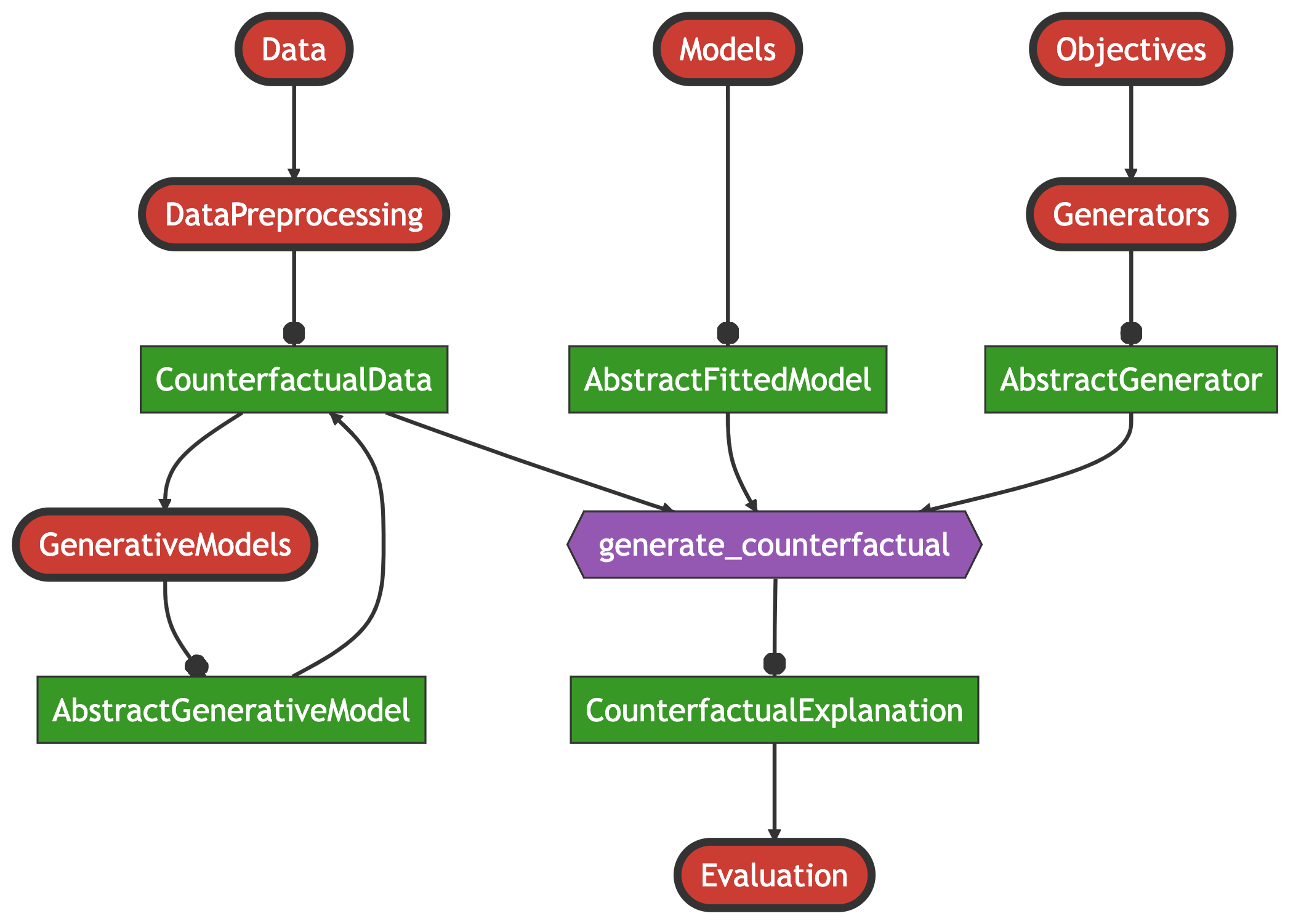
3.1 Models

The package currently offers native support for models built and trained in Flux (Innes 2018) as well as a small subset of models made available through MLJ (Blaom et al. 2020). While in general it is assumed that users resort to this package to explain their pre-trained models, we provide a simple API call to train the following models:

• Linear Classifier (Logistic Regression and Multinomial Logit)
• Multi-Layer Perceptron (Deep Neural Network)
• Deep Ensemble Lakshminarayanan, Pritzel, and Blundell (2016)
• Decision Tree, Random Forest, Gradient Boosted Trees

As we demonstrate below, it is straightforward to extend the package through custom models. Support for torch models trained in Python or R is also available.⁴

3.2 Generators

A large and growing number of counterfactual generators have already been implemented in our package (Table 1). At a high level, we distinguish generators in terms of their compatible model types, their default search space, and their composability. All “gradient-based” generators are compatible with differentiable models, e.g. Flux and torch, while “tree-based” generators are only applicable to models that involve decision trees. Concerning the search space, it is possible to search counterfactuals in a lower-dimensional latent embedding of the feature space that implicitly encodes the data-generating process (DGP). To learn the latent embedding, existing work has typically relied on generative models or existing causal knowledge (Joshi et al. 2019; Karimi, Schölkopf, and Valera 2021). While this notion is compatible with all of our gradient-based generators, only some generators search a latent space by default. Finally, composability implies that the given generator can be blended with any other composable generator, which we discuss in Section 4.2.

Beyond these broad technical distinctions, generators largely differ in terms of how they address the various desiderata mentioned above: ClapROAR aims to preserve the classifier, i.e. to generate counterfactuals that are robust to endogenous model shifts (Altmeyer et al. 2023); CLUE searches plausible counterfactuals in the latent embedding of a generative model by explicitly minimising predictive entropy (Antorán et al. 2020); DiCE is designed to generate multiple, maximally diverse counterfactuals (Mothilal, Sharma, and Tan 2020); FeatureTweak leverages the internals of decision trees to search counterfactuals on a feature-by-feature basis, finding the counterfactual that tweaks the features in the least costly way (Tolomei et al. 2017); Gravitational aims to generate plausible and robust counterfactuals by minimising the distance to observed samples in the target class (Altmeyer et al. 2023); Greedy aims to generate plausible counterfactuals by implicitly minimising predictive uncertainty of Bayesian classifiers (Schut et al. 2021); GrowingSpheres is model-agnostic, relying solely on identifying nearest neighbours of counterfactuals in the target class by gradually increasing the search radius and then moving counterfactuals in that direction(Laugel et al. 2017); PROBE generates probabilistically robust counterfactuals (Pawelczyk et al. 2022); REVISE addresses the need for plausibility by searching counterfactuals in the latent embedding of a Variational Autoencoder (VAE) (Joshi et al. 2019); Wachter is the baseline approach that only penalises the distance to the original sample (Wachter, Mittelstadt, and Russell 2017).

Table 1: Overview of implemented counterfactual generators.

Generator	Model Type	Search Space	Composable
ClaPROAR (Altmeyer et al. 2023)	gradient based	feature	yes
CLUE (Antorán et al. 2020)	gradient based	latent	yes
DiCE (Mothilal, Sharma, and Tan 2020)	gradient based	feature	yes
FeatureTweak (Tolomei et al. 2017)	tree based	feature	no
Gravitational (Altmeyer et al. 2023)	gradient based	feature	yes
Greedy (Schut et al. 2021)	gradient based	feature	yes
GrowingSpheres (Laugel et al. 2017)	agnostic	feature	no
PROBE (Pawelczyk et al. 2022)	gradient based	feature	no
REVISE (Joshi et al. 2019)	gradient based	latent	yes
Wachter (Wachter, Mittelstadt, and Russell 2017)	gradient based	feature	yes

3.3 Data Catalogue

To allow researchers and practitioners to test and compare counterfactual generators, the package ships with catalogues of pre-processed synthetic and real-world benchmark datasets from different domains. Real-world datasets include:

• Adult Census (Barry Becker 1996)
• California Housing (Pace and Barry 1997)
• CIFAR10 (Krizhevsky 2009)
• German Credit (Hoffman 1994)
• Give Me Some Credit (Kaggle 2011)
• MNIST (LeCun 1998) and Fashion MNIST (Xiao, Rasul, and Vollgraf 2017)
• UCI defaultCredit (Yeh and Lien 2009)

Custom datasets can also be easily preprocessed as explained in the documentation.

3.4 Plotting

The package also extends common Plots.jl methods to facilitate the visualization of results. Calling the generic plot() method on an instance of type <:CounterfactualExplanation, for example, generates a plot visualizing the entire counterfactual path in the feature space⁵. We will see several examples of this below.

4 Basic Usage

In the following, we begin our exploration of the package functionality with a simple example. We then demonstrate how more advanced generators can be easily composed and show how users can impose mutability constraints on features. Finally, we also briefly explore the topics of counterfactual evaluation and benchmarking.

4.1 A Simple Generic Generator

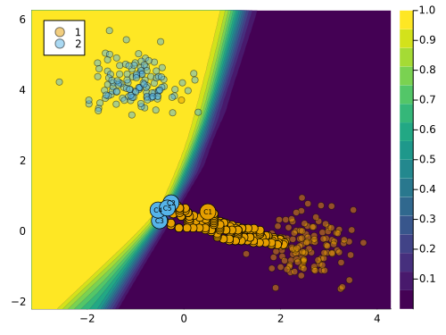
Code \(\ref{lst:simple}\) below provides a complete example demonstrating how the framework presented in Section 2.2 can be implemented through our package. Using a synthetic data set with linearly separable features we first fit a linear classifier (line \(\ref{line:simple-class}\)). Next, we define the target class (line \(\ref{line:simple-t}\)) and then draw a random sample from the other class (line \(\ref{line:simple-x}\)). Finally, we instantiate a generic generator (line \(\ref{line:simple-gen}\)) and run the counterfactual search (line \(\ref{line:simple-search}\)). Figure 2 illustrates the resulting counterfactual path in the two-dimensional feature space. Features go through iterative perturbations until the desired confidence level is reached as illustrated by the contour in the background, which shows the softmax output for the target class.

Figure 2: Counterfactual path using generic counterfactual generator for conventional binary classifier.

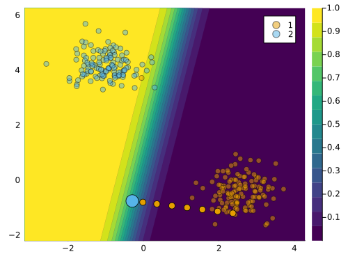
In this simple example, the generic generator produces a valid counterfactual, since the decision boundary is crossed and the predicted label is flipped. But the counterfactual is not plausible: it does not appear to be generated by the same DGP as the observed data in the target class. This is because the generic generator does not take into account any of the desiderata mentioned in Section 2.2, except for the distance to the factual sample.

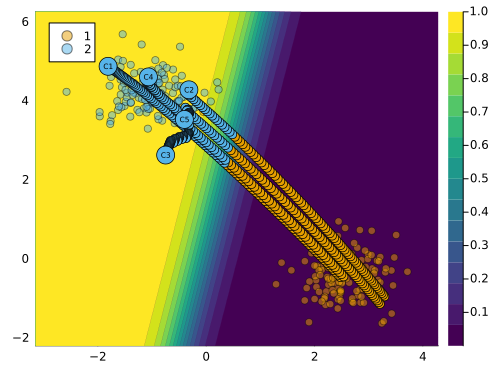
4.2 Composing Generators

To address these issues, we can leverage the ideas underlying some of the more advanced counterfactual generators introduced above. In particular, we will now show how easy it is to compose custom generators that blend different ideas through user-friendly macros.

Suppose we wanted to address the desiderata of plausibility and diversity. We could do this by blending ideas underlying the DiCE generator with the REVISE generator. Formally, the corresponding search objective would be defined as follows,

\[ \mathbf{Z}^\prime = \arg \min_{\mathbf{Z}^\prime \in \mathcal{Z}^{L \times K}} \{ {\ell(M(f(\mathbf{Z}^\prime)),t)} + \lambda \cdot {\text{diversity}(f(\mathbf{Z}^\prime)) } \} \tag{3}\]

where \(\mathbf{X}^\prime\) is an \(L\)-dimensional array of counterfactuals, \(f: \mathcal{Z}^{L \times K} \mapsto \mathcal{X}^{L \times D}\) is a function that maps the \(L \times K\)-dimensional latent space \(\mathcal{Z}\) to the \(L \times D\)-dimensional feature space \(\mathcal{X}\) and \(\text{diversity}(\cdot)\) is the penalty proposed by Mothilal, Sharma, and Tan (2020) that induces diverse sets of counterfactuals. As in Equation 2, \(\ell\) is the loss function, \(M\) is the black-box model, \(t\) is the target class, and \(\lambda\) is the strength of the penalty.

Code \(\ref{lst:composed}\) demonstrates how Equation 3 can be seamlessly translated into Julia code. We begin by instantiating a GradientBasedGenerator in line \(\ref{line:composed-init}\). Next, we use chained macros for composition: firstly, we define the counterfactual search @objective corresponding to DiCE in line \(\ref{line:composed-dice}\); secondly, we define the latent space search strategy corresponding to REVISE using the @search_latent_space macro in line \(\ref{line:composed-latent}\); finally, we specify our prefered optimisation method using the @with_optimiser macro in line \(\ref{line:composed-adam}\).

In this case, the counterfactual search is performed in the latent space of a Variational Autoencoder (VAE) that is automatically trained on the observed data. It is important to specify the keyword argument num_counterfactuals of the generate_counterfactual to some value higher than \(1\) (default), to ensure that the diversity penalty is effective. The resulting counterfactual path is shown in Figure 3 below. We observe that the resulting counterfactuals are diverse and the majority of them are plausible.

Figure 3: Counterfactual path using the DiCE generator.

4.3 Mutability Constraints

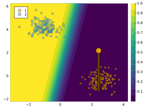
In practice, features usually cannot be perturbed arbitrarily. Suppose, for example, that one of the features used by a bank to predict the creditworthiness of its clients is age. If a counterfactual explanation for the prediction model indicates that older clients should “grow younger” to improve their creditworthiness, then this is an interesting insight (it reveals age bias), but the provided recourse is not actionable. In such cases, we may want to constrain the mutability of features. To illustrate how this can be implemented in our package, we will continue with the example from above.

Mutability can be defined in terms of four different options: 1) the feature is mutable in both directions, 2) the feature can only increase (e.g. age), 3) the feature can only decrease (e.g. time left until your next deadline) and 4) the feature is not mutable (e.g. skin colour, ethnicity, …). To specify which category a feature belongs to, users can pass a vector of symbols containing the mutability constraints at the pre-processing stage. For each feature one can choose from these four options: :both (mutable in both directions), :increase (only up), :decrease (only down) and :none (immutable). By default, nothing is passed to that keyword argument and it is assumed that all features are mutable in both directions.⁶

We can impose that the first feature is immutable as follows: counterfactual_data.mutability = [:none, :both]. The resulting counterfactual path is shown in Figure 4 below. Since only the second feature can be perturbed, the sample can only move along the vertical axis. In this case, the counterfactual search does not yield a valid counterfactual, since the target class is not reached.

Figure 4: Counterfactual path with immutable feature.

4.4 Evaluation and Benchmarking

The package also makes it easy to evaluate counterfactuals with respect to many of the desiderata mentioned above. For example, users may want to infer how costly the provided recourse is to individuals. To this end, we can measure the distance of the counterfactual from its original value. The API call to compute the distance metric defined in Wachter, Mittelstadt, and Russell (2017), for instance, is as simple as evaluate(ce; measure=distance_mad), where ce can also be a vector of CounterfactualExplanations.

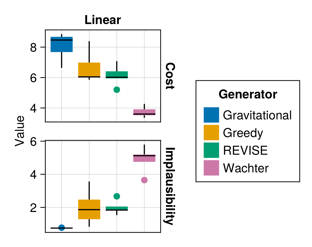
Additionally, the package provides a benchmarking framework that allows users to compare the performance of different generators on a given dataset. In Figure 5 we show the results of a benchmark comparing several generators in terms of the average cost and implausibility of the generated counterfactuals. The cost is proxied by the L1-norm of the difference between the factual and counterfactual features, while implausibility is measured by the distance of the counterfactuals from samples in the target class. The results illustrate that there is a tradeoff between minimizing costs to individuals and generating plausible counterfactuals.

Figure 5: Benchmarking results for different generators.

5 Customization and Extensibility

One of our priorities has been to make our package customizable and extensible. In the long term, we aim to add support for more default models and counterfactual generators. In the short term, it is designed to allow users to integrate models and generators themselves. These community efforts will facilitate our long-term goals.

5.1 Adding Custom Models

At the high level, only two steps are necessary to make any supervised learning model compatible with our package:

• : We need to subtype the .
• : The functions and need to be extended through custom methods for the model in question.

To demonstrate how this can be done in practice, we will reiterate here how native support for Flux.jl (Innes 2018) deep learning models was enabled.⁷ Once again we use synthetic data for an illustrative example. Code \(\ref{lst:nn}\) below builds a simple model architecture that can be used for a multi-class prediction task. Note how outputs from the final layer are not passed through a softmax activation function, since the counterfactual loss is evaluated with respect to logits as we discussed earlier. The model is trained with dropout.

Code \(\ref{lst:mymodel}\) below implements the two steps that were necessary to make Flux models compatible with the package. In line \(\ref{line:mymodel-subtype}\) we declare our new struct as a subtype of AbstractDifferentiableModel, which itself is an abstract subtype of AbstractFittedModel.⁸ Computing logits amounts to just calling the model on inputs. Predicted probabilities for labels can be computed by passing logits through the softmax function.

The API call for generating counterfactuals for our new model is the same as before. Figure 6 shows the resulting counterfactual path for a randomly chosen sample. In this case, the contour shows the predicted probability that the input is in the target class (\(t=2\)).

Figure 6: Counterfactual path using generic counterfactual generator for multi-class classifier.

5.2 Adding Custom Generators

In some cases, composability may not be sufficient to implement specific logics underlying certain counterfactual generators. In such cases, users may want to implement custom generators. To illustrate how this can be done we will consider a simple extension of our GenericGenerator. As we have seen above, Counterfactual Explanations are not unique. In light of this, we might be interested in quantifying the uncertainty around the generated counterfactuals (Delaney, Greene, and Keane 2021). One idea could be, to use dropout to randomly switch features on and off in each iteration. Without dwelling further on the merit of this idea, we will now briefly show how this can be implemented.

5.2.1 A Generator with Dropout

Code \(\ref{lst:dropout}\) below implements two important steps: 1) create an abstract subtype of the AbstractGradientBasedGenerator and 2) create a constructor with an additional field for the dropout probability.

Next, in Code \(\ref{lst:generate}\) we define how feature perturbations are generated for our custom dropout generator: in particular, we extend the relevant function through a method that implements the dropout logic.

Finally, we proceed to generate counterfactuals in the same way we always do. The resulting counterfactual path is shown in Figure 7.

Figure 7: Counterfactual path for a generator with dropout.

6 A Real-World Examples

Now that we have explained the basic functionality of CounterfactualExplanations.jl through some synthetic examples, it is time to work through examples involving real-world data.

6.1 Give Me Some Credit

The Give Me Some Credit dataset is one of the tabular real-world datasets that ship with the package (Kaggle 2011). It can be used to train a binary classifier to predict whether a borrower is likely to experience financial difficulties in the next two years. In particular, we have an output variable \(y \in \{0=\texttt{no stress},1=\texttt{stress}\}\) and a feature matrix \(X\) that includes socio-demographic variables like age and income. A retail bank might use such a classifier to determine if potential borrowers should receive credit or not.

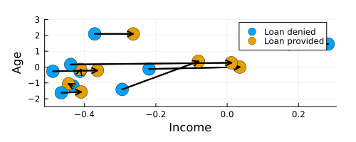
For the classification task, we use a Multi-Layer Perceptron with dropout regularization. Using the Gravitational generator (Altmeyer et al. 2023) we will generate counterfactuals for ten randomly chosen individuals that would be denied credit based on our pre-trained model. Concerning the mutability of features, we only impose that the age cannot be decreased.

Figure 8 shows the resulting counterfactuals proposed by Wachter in the two-dimensional feature space spanned by the age and income variables. An increase in income and age is recommended for the majority of individuals, which seems plausible: both age and income are typically positively related to creditworthiness.

Figure 8: Give Me Some Credit: counterfactuals for would-be borrowers proposed by the Gravitational Generator.

6.2 MNIST

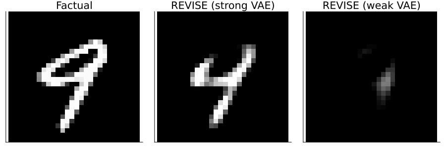
For our second example, we will look at image data. The MNIST dataset contains 60,000 training samples of handwritten digits in the form of 28x28 pixel grey-scale images (LeCun 1998). Each image is associated with a label indicating the digit (0-9) that the image represents. The data makes for an interesting case study of CE because humans have a good idea of what plausible counterfactuals of digits look like. For example, if you were asked to pick up an eraser and turn the digit in the left panel of Figure 9 into a four (4) you would know exactly what to do: just erase the top part.

On the model side, we will use a simple multi-layer perceptron (MLP). Code \(\ref{lst:mnist-setup}\) loads the data and the pre-trained MLP. It also loads two pre-trained Variational Auto-Encoders, which will be used by our counterfactual generator of choice for this task: REVISE.

The proposed counterfactuals are shown in Figure 9. In the case in which REVISE has access to an expressive VAE (centre), the result looks convincing: the perturbed image does look like it represents a four (4). In terms of explainability, we may conclude that removing the top part of the handwritten nine (9) leads the black-box model to predict that the perturbed image represents a four (4). We should note, however, that the quality of counterfactuals produced by REVISE hinges on the performance of the underlying generative model, as demonstrated by the result on the right. In this case, REVISE uses a weak VAE and the resulting counterfactual is invalid. In light of this, we recommend using Latent Space search with care.

Figure 9: Counterfactual explanations for MNIST using a Latent Space generator: turning a nine (9) into a four (4).

7 Discussion and Outlook

We believe that this package in its current form offers a valuable contribution to ongoing efforts towards XAI in Julia. That being said, there is significant scope for future developments, which we briefly outline in this final section.

7.1 Candidate models and generators

The package supports various models and generators either natively or through minimal augmentation. In future work, we would like to prioritize the addition of further predictive models and generators. Concerning the former, it would be useful to add native support for any supervised models built in MLJ.jl, an extensive Machine Learning framework for Julia (Blaom et al. 2020). This may also involve adding support for regression models as well as additional non-differentiable models. In terms of counterfactual generators, there is a list of recent methodologies that we would like to implement including MINT (Karimi, Schölkopf, and Valera 2021), ROAR (Upadhyay, Joshi, and Lakkaraju 2021) and FACE (Poyiadzi et al. 2020).

7.2 Additional datasets

For benchmarking and testing purposes it will be crucial to add more datasets to our library. We have so far prioritized tabular datasets that have typically been used in the literature on counterfactual explanations including Adult, Give Me Some Credit and German Credit (Karimi, Barthe, et al. 2020). There is scope for adding data sources that have so far not been explored much in this context including additional image datasets as well as audio, natural language and time-series data.

8 Concluding remarks

CounterfactualExplanation.jl is a package for generating Counterfactual Explanations and Algorithmic Recourse in Julia. Through various synthetic and real-world examples, we have demonstrated the basic usage of the package as well as its extensibility. The package has already served us in our research to benchmark various methodological approaches to Counterfactual Explanations and Algorithmic Recourse. We therefore strongly believe that it should help other practitioners and researchers in their own efforts towards Trustworthy AI.

We envision this package to one day constitute the go-to place for explaining arbitrary predictive models through an extensive suite of counterfactual generators. As a major next step, we aim to make our library as compatible as possible with the popular MLJ.jl package for machine learning in Julia. We invite the Julia community to contribute to these goals through usage, open challenge and active development.

9 Acknowledgements

We are immensely grateful to the group of TU Delft students who contributed huge improvements to this package as part of a university project in 2023: Rauno Arike, Simon Kasdorp, Lauri Kesküll, Mariusz Kicior, Vincent Pikand. We also want to thank the broader Julia community for being welcoming and open and for supporting research contributions like this one. Some of the members of TU Delft were partially funded by ICAI AI for Fintech Research, an ING—TU Delft collaboration.

10 References

Altmeyer, Patrick, Giovan Angela, Aleksander Buszydlik, Karol Dobiczek, Arie van Deursen, and Cynthia Liem. 2023. “Endogenous Macrodynamics in Algorithmic Recourse.” In First IEEE Conference on Secure and Trustworthy Machine Learning. https://doi.org/10.1109/satml54575.2023.00036.

Antorán, Javier, Umang Bhatt, Tameem Adel, Adrian Weller, and José Miguel Hernández-Lobato. 2020. “Getting a Clue: A Method for Explaining Uncertainty Estimates.” https://arxiv.org/abs/2006.06848.

Arrieta, Alejandro Barredo, Natalia Diaz-Rodriguez, Javier Del Ser, Adrien Bennetot, Siham Tabik, Alberto Barbado, Salvador Garcia, et al. 2020. “Explainable Artificial Intelligence (XAI): Concepts, Taxonomies, Opportunities and Challenges Toward Responsible AI.” Information Fusion 58: 82–115. https://doi.org/10.1016/j.inffus.2019.12.012.

Barry Becker, Ronny Kohavi. 1996. “Adult.” UCI Machine Learning Repository. https://doi.org/10.24432/C5XW20.

Blaom, Anthony D., Franz Kiraly, Thibaut Lienart, Yiannis Simillides, Diego Arenas, and Sebastian J. Vollmer. 2020. “MLJ: A Julia Package for Composable Machine Learning.” Journal of Open Source Software 5 (55): 2704. https://doi.org/10.21105/joss.02704.

Borch, Christian. 2022. “Machine Learning, Knowledge Risk, and Principal-Agent Problems in Automated Trading.” Technology in Society, 101852. https://doi.org/10.1016/j.techsoc.2021.101852.

Buolamwini, Joy, and Timnit Gebru. 2018. “Gender Shades: Intersectional Accuracy Disparities in Commercial Gender Classification.” In Conference on Fairness, Accountability and Transparency, 77–91. PMLR.

Dandl, Susanne, Andreas Hofheinz, Martin Binder, Bernd Bischl, and Giuseppe Casalicchio. 2023. “Counterfactuals: An R Package for Counterfactual Explanation Methods.” arXiv. http://arxiv.org/abs/2304.06569.

Delaney, Eoin, Derek Greene, and Mark T. Keane. 2021. “Uncertainty Estimation and Out-of-Distribution Detection for Counterfactual Explanations: Pitfalls and Solutions.” arXiv. http://arxiv.org/abs/2107.09734.

Fan, Fenglei, Jinjun Xiong, and Ge Wang. 2020. “On Interpretability of Artificial Neural Networks.” https://arxiv.org/abs/2001.02522.

Goodfellow, Ian J, Jonathon Shlens, and Christian Szegedy. 2014. “Explaining and Harnessing Adversarial Examples.” https://arxiv.org/abs/1412.6572.

Hoffman, Hans. 1994. “German Credit Data.” https://archive.ics.uci.edu/ml/datasets/statlog+(german+credit+data).

Innes, Mike. 2018. “Flux: Elegant Machine Learning with Julia.” Journal of Open Source Software 3 (25): 602. https://doi.org/10.21105/joss.00602.

Joshi, Shalmali, Oluwasanmi Koyejo, Warut Vijitbenjaronk, Been Kim, and Joydeep Ghosh. 2019. “Towards Realistic Individual Recourse and Actionable Explanations in Black-Box Decision Making Systems.” https://arxiv.org/abs/1907.09615.

Kaggle. 2011. “Give Me Some Credit, Improve on the State of the Art in Credit Scoring by Predicting the Probability That Somebody Will Experience Financial Distress in the Next Two Years.” Kaggle. https://www.kaggle.com/c/GiveMeSomeCredit.

Karimi, Amir-Hossein, Gilles Barthe, Bernhard Schölkopf, and Isabel Valera. 2020. “A Survey of Algorithmic Recourse: Definitions, Formulations, Solutions, and Prospects.” https://arxiv.org/abs/2010.04050.

Karimi, Amir-Hossein, Bernhard Schölkopf, and Isabel Valera. 2021. “Algorithmic Recourse: From Counterfactual Explanations to Interventions.” In Proceedings of the 2021 ACM Conference on Fairness, Accountability, and Transparency, 353–62.

Karimi, Amir-Hossein, Julius Von Kügelgen, Bernhard Schölkopf, and Isabel Valera. 2020. “Algorithmic Recourse Under Imperfect Causal Knowledge: A Probabilistic Approach.” https://arxiv.org/abs/2006.06831.

Kaur, Harmanpreet, Harsha Nori, Samuel Jenkins, Rich Caruana, Hanna Wallach, and Jennifer Wortman Vaughan. 2020. “Interpreting Interpretability: Understanding Data Scientists’ Use of Interpretability Tools for Machine Learning.” In Proceedings of the 2020 CHI Conference on Human Factors in Computing Systems, 1–14. https://doi.org/10.1145/3313831.3376219.

Krizhevsky, A. 2009. “Learning Multiple Layers of Features from Tiny Images.” In. https://www.semanticscholar.org/paper/Learning-Multiple-Layers-of-Features-from-Tiny-Krizhevsky/5d90f06bb70a0a3dced62413346235c02b1aa086.

Lakshminarayanan, Balaji, Alexander Pritzel, and Charles Blundell. 2016. “Simple and Scalable Predictive Uncertainty Estimation Using Deep Ensembles.” https://arxiv.org/abs/1612.01474.

Laugel, Thibault, Marie-Jeanne Lesot, Christophe Marsala, Xavier Renard, and Marcin Detyniecki. 2017. “Inverse Classification for Comparison-Based Interpretability in Machine Learning.” arXiv. https://doi.org/10.48550/arXiv.1712.08443.

LeCun, Yann. 1998. “The MNIST Database of Handwritten Digits.”

Miller, Tim. 2019. “Explanation in Artificial Intelligence: Insights from the Social Sciences.” Artificial Intelligence 267: 1–38. https://doi.org/10.1016/j.artint.2018.07.007.

Molnar, Christoph. 2020. Interpretable Machine Learning. Lulu. com.

Mothilal, Ramaravind K, Amit Sharma, and Chenhao Tan. 2020. “Explaining Machine Learning Classifiers Through Diverse Counterfactual Explanations.” In Proceedings of the 2020 Conference on Fairness, Accountability, and Transparency, 607–17. https://doi.org/10.1145/3351095.3372850.

O’Neil, Cathy. 2016. Weapons of Math Destruction: How Big Data Increases Inequality and Threatens Democracy. Crown.

Pace, R Kelley, and Ronald Barry. 1997. “Sparse Spatial Autoregressions.” Statistics & Probability Letters 33 (3): 291–97. https://doi.org/10.1016/s0167-7152(96)00140-x.

Pawelczyk, Martin, Sascha Bielawski, Johannes van den Heuvel, Tobias Richter, and Gjergji Kasneci. 2021. “Carla: A Python Library to Benchmark Algorithmic Recourse and Counterfactual Explanation Algorithms.” https://arxiv.org/abs/2108.00783.

Pawelczyk, Martin, Teresa Datta, Johannes van-den-Heuvel, Gjergji Kasneci, and Himabindu Lakkaraju. 2022. “Probabilistically Robust Recourse: Navigating the Trade-Offs Between Costs and Robustness in Algorithmic Recourse.” arXiv Preprint arXiv:2203.06768.

Poyiadzi, Rafael, Kacper Sokol, Raul Santos-Rodriguez, Tijl De Bie, and Peter Flach. 2020. “FACE: Feasible and Actionable Counterfactual Explanations.” In Proceedings of the AAAI/ACM Conference on AI, Ethics, and Society, 344–50.

Rudin, Cynthia. 2019. “Stop Explaining Black Box Machine Learning Models for High Stakes Decisions and Use Interpretable Models Instead.” Nature Machine Intelligence 1 (5): 206–15. https://doi.org/10.1038/s42256-019-0048-x.

Schut, Lisa, Oscar Key, Rory Mc Grath, Luca Costabello, Bogdan Sacaleanu, Yarin Gal, et al. 2021. “Generating Interpretable Counterfactual Explanations By Implicit Minimisation of Epistemic and Aleatoric Uncertainties.” In International Conference on Artificial Intelligence and Statistics, 1756–64. PMLR.

Slack, Dylan, Anna Hilgard, Himabindu Lakkaraju, and Sameer Singh. 2021. “Counterfactual Explanations Can Be Manipulated.” Advances in Neural Information Processing Systems 34.

Slack, Dylan, Sophie Hilgard, Emily Jia, Sameer Singh, and Himabindu Lakkaraju. 2020. “Fooling Lime and Shap: Adversarial Attacks on Post Hoc Explanation Methods.” In Proceedings of the AAAI/ACM Conference on AI, Ethics, and Society, 180–86.

Tolomei, Gabriele, Fabrizio Silvestri, Andrew Haines, and Mounia Lalmas. 2017. “Interpretable Predictions of Tree-Based Ensembles via Actionable Feature Tweaking.” In Proceedings of the 23rd ACM SIGKDD International Conference on Knowledge Discovery and Data Mining, 465–74. https://doi.org/10.1145/3097983.3098039.

Upadhyay, Sohini, Shalmali Joshi, and Himabindu Lakkaraju. 2021. “Towards Robust and Reliable Algorithmic Recourse.” https://arxiv.org/abs/2102.13620.

Ustun, Berk, Alexander Spangher, and Yang Liu. 2019. “Actionable Recourse in Linear Classification.” In Proceedings of the Conference on Fairness, Accountability, and Transparency, 10–19. https://doi.org/10.1145/3287560.3287566.

Varshney, Kush R. 2022. Trustworthy Machine Learning. Chappaqua, NY, USA: Independently Published.

Verma, Sahil, John Dickerson, and Keegan Hines. 2020. “Counterfactual Explanations for Machine Learning: A Review.” https://arxiv.org/abs/2010.10596.

Wachter, Sandra, Brent Mittelstadt, and Chris Russell. 2017. “Counterfactual Explanations Without Opening the Black Box: Automated Decisions and the GDPR.” Harv. JL & Tech. 31: 841. https://doi.org/10.2139/ssrn.3063289.

Xiao, Han, Kashif Rasul, and Roland Vollgraf. 2017. “Fashion-MNIST: A Novel Image Dataset for Benchmarking Machine Learning Algorithms.” arXiv. https://doi.org/10.48550/arXiv.1708.07747.

Yeh, I-Cheng, and Che-hui Lien. 2009. “The Comparisons of Data Mining Techniques for the Predictive Accuracy of Probability of Default of Credit Card Clients.” Expert Systems with Applications 36 (2): 2473–80. https://doi.org/10.1016/j.eswa.2007.12.020.

Footnotes

1. Implementations of loss functions with respect to logits are often numerically more stable. For example, the logitbinarycrossentropy(ŷ, y) implementation in Flux.Losses (used here) is more stable than the mathematically equivalent binarycrossentropy(ŷ, y).

2. While we were writing this paper, the R package counterfactuals was released (Dandl et al. 2023). The developers seem to also envision a unifying framework, but the project appears to still be in its early stages.

3. For details, see the Google Summer of Code 2022 project proposal: https://julialang.org/jsoc/gsoc/MLJ/#interpretable_machine_learning_in_julia.

4. We are currently relying on PythonCall.jl and RCall.jl and this functionality is still somewhat brittle. Since this is more of an edge case, we may move this feature into its own package in the future.

5. For multi-dimensional input data, standard dimensionality reduction techniques are used to compress the data. In this case, the classifier’s decision boundary is approximated through a Nearest Neighbour model. This is still somewhat experimental and will be improved in the future.

6. Mutability constraints are not yet implemented for Latent Space search.

7. Flux models are now natively supported by our package and can be instantiated by calling FluxModel().

8. Note that in line \(\ref{line:mymodel-likelihood}\) we also provide a field determining the likelihood. This is optional and only used internally to determine which loss function to use in the counterfactual search. If this field is not provided to the model, the loss function needs to be explicitly supplied to the generator.