4 Faithful Model Explanations through Energy-Constrained Conformal Counterfactuals
Counterfactual explanations offer an intuitive and straightforward way to explain black-box models and offer algorithmic recourse to individuals. To address the need for plausible explanations, existing work has primarily relied on surrogate models to learn how the input data is distributed. This effectively reallocates the task of learning realistic explanations for the data from the model itself to the surrogate. Consequently, the generated explanations may seem plausible to humans but need not necessarily describe the behavior of the black-box model faithfully. We formalize this notion of faithfulness through the introduction of a tailored evaluation metric and propose a novel algorithmic framework for generating Energy-Constrained Conformal Counterfactuals that are only as plausible as the model permits. Through extensive empirical studies, we demonstrate that ECCCo reconciles the need for faithfulness and plausibility. In particular, we show that for models with gradient access, it is possible to achieve state-of-the-art performance without the need for surrogate models. To do so, our framework relies solely on properties defining the black-box model itself by leveraging recent advances in energy-based modelling and conformal prediction. To our knowledge, this is the first venture in this direction for generating faithful counterfactual explanations. Thus, we anticipate that ECCCo can serve as a baseline for future research. We believe that our work opens avenues for researchers and practitioners seeking tools to better distinguish trustworthy from unreliable models.
Explainable ML, Counterfactual Explanations, Faithfulness, Algorithmic Recourse, Energy-Based Models
4.1 Introduction
Counterfactual explanations provide a powerful, flexible and intuitive way to not only explain black-box models but also offer the possibility of algorithmic recourse to affected individuals. Instead of opening the black box, counterfactual explanations work under the premise of strategically perturbing model inputs to understand model behavior (Wachter, Mittelstadt, and Russell 2017). Intuitively speaking, we generate explanations in this context by asking what-if questions of the following nature: ‘Our credit risk model currently predicts that this individual is not credit-worthy. What if they reduced their monthly expenditures by 10%?’
This is typically implemented by defining a target outcome \(\mathbf{y}^+ \in \mathcal{Y}\) for some individual \(\mathbf{x} \in \mathcal{X}=\mathbb{R}^D\) described by \(D\) attributes, for which the model \(M_{\theta}:\mathcal{X}\mapsto\mathcal{Y}\) initially predicts a different outcome: \(M_{\theta}(\mathbf{x})\ne \mathbf{y}^+\). Counterfactuals are then searched by minimizing a loss function that compares the predicted model output to the target outcome: \(\text{yloss}(M_{\theta}(\mathbf{x}),\mathbf{y}^+)\). Since counterfactual explanations work directly with the black-box model, valid counterfactuals always have full local fidelity by construction where fidelity is defined as the degree to which explanations approximate the predictions of a black-box model (Molnar 2022).
In situations where full fidelity is a requirement, counterfactual explanations offer a more appropriate solution to Explainable Artificial Intelligence (XAI) than other popular approaches like LIME (Ribeiro, Singh, and Guestrin 2016) and SHAP (Lundberg and Lee 2017), which involve local surrogate models. But even full fidelity is not a sufficient condition for ensuring that an explanation faithfully describes the behavior of a model. That is because multiple distinct explanations can lead to the same model prediction, especially when dealing with heavily parameterized models like deep neural networks, which are underspecified by the data (Wilson 2020). In the context of counterfactuals, the idea that no two explanations are the same arises almost naturally. A key focus in the literature has therefore been to identify those explanations that are most appropriate based on a myriad of desiderata such as closeness (Wachter, Mittelstadt, and Russell 2017), sparsity (Schut et al. 2021), actionability (Ustun, Spangher, and Liu 2019) and plausibility (Joshi et al. 2019).
In this work, we draw closer attention to modelling faithfulness rather than fidelity as a desideratum for counterfactuals. We define faithfulness as the degree to which counterfactuals are consistent with what the model has learned about the data. Our key contributions are as follows: first, we show that fidelity is an insufficient evaluation metric for counterfactuals (Section 4.3) and propose a definition of faithfulness that gives rise to more suitable metrics (Section 4.4). Next, we introduce a ECCCo: a novel algorithmic approach aimed at generating energy-constrained conformal counterfactuals that faithfully explain model behavior in Section 4.5. Finally, we provide extensive empirical evidence demonstrating that ECCCo faithfully explains model behavior and attains plausibility only when appropriate (Section 4.6).
To our knowledge, this is the first venture in this direction for generating faithful counterfactuals. Thus, we anticipate that ECCCo can serve as a baseline for future research. We believe that our work opens avenues for researchers and practitioners seeking tools to better distinguish trustworthy from unreliable models.
4.2 Background
While counterfactual explanations (CE) can also be generated for arbitrary regression models (Spooner et al. 2021), existing work has primarily focused on classification problems. Let \(\mathcal{Y}=(0,1)^K\) denote the one-hot-encoded output domain with \(K\) classes. Then most counterfactual generators rely on gradient descent to optimize different flavors of the following counterfactual search objective:
\[ \begin{aligned} \min_{\mathbf{Z}^\prime \in \mathcal{Z}^L} \left\{ {\text{yloss}(M_{\theta}(f(\mathbf{Z}^\prime)),\mathbf{y}^+)}+ \lambda {\text{cost}(f(\mathbf{Z}^\prime)) } \right\} \end{aligned} \tag{4.1}\]
Here \(\text{yloss}(\cdot)\) denotes the primary loss function, \(f(\cdot)\) is a function that maps from the counterfactual state space to the feature space and \(\text{cost}(\cdot)\) is either a single penalty or a collection of penalties that are used to impose constraints through regularization. Equation 5.1 restates the baseline approach to gradient-based counterfactual search proposed by Wachter, Mittelstadt, and Russell (2017) in general form as introduced Chapter 2. To explicitly account for the multiplicity of explanations, \(\mathbf{Z}^\prime=\{ \mathbf{z}_l\}_L\) denotes an \(L\)-dimensional array of counterfactual states.
The baseline approach, which we will simply refer to as Wachter, searches a single counterfactual directly in the feature space and penalizes its distance to the original factual. In this case, \(f(\cdot)\) is simply the identity function and \(\mathcal{Z}\) corresponds to the feature space itself. Many derivative works of Wachter, Mittelstadt, and Russell (2017) have proposed new flavors of Equation 5.1, each of them designed to address specific desiderata that counterfactuals ought to meet in order to properly serve both AI practitioners and individuals affected by algorithmic decision-making systems. The list of desiderata includes but is not limited to the following: sparsity, closeness (Wachter, Mittelstadt, and Russell 2017), actionability (Ustun, Spangher, and Liu 2019), diversity (Mothilal, Sharma, and Tan 2020), plausibility (Joshi et al. 2019; Poyiadzi et al. 2020; Schut et al. 2021), robustness (Upadhyay, Joshi, and Lakkaraju 2021; Pawelczyk et al. 2023; Altmeyer et al. 2023) and causality (Karimi, Schölkopf, and Valera 2021). Different counterfactual generators addressing these needs have been extensively surveyed and evaluated in various studies (Verma et al. 2022; Karimi et al. 2021; Pawelczyk et al. 2021; Artelt et al. 2021; Guidotti 2022).
The notion of plausibility is central to all of the desiderata. For example, Artelt et al. (2021) find that plausibility typically also leads to improved robustness. Similarly, plausibility has also been connected to causality in the sense that plausible counterfactuals respect causal relationships (Mahajan, Tan, and Sharma 2020). Consequently, the plausibility of counterfactuals has been among the primary concerns for researchers. Achieving plausibility is equivalent to ensuring that the generated counterfactuals comply with the true and unobserved data-generating process (DGP). We define plausibility formally in this work as follows:
Definition 4.1 (Plausible Counterfactuals) Let \(\mathcal{X}|\mathbf{y}^+= p(\mathbf{x}|\mathbf{y}^+)\) denote the true conditional distribution of samples in the target class \(\mathbf{y}^+\). Then for \(\mathbf{x}^{\prime}\) to be considered a plausible counterfactual, we need: \(\mathbf{x}^{\prime} \sim \mathcal{X}|\mathbf{y}^+\).
To generate plausible counterfactuals, we first need to quantify the conditional distribution of samples in the target class (\(\mathcal{X}|\mathbf{y}^+\)). We can then ensure that we generate counterfactuals that comply with that distribution.
One straightforward way to do this is to use surrogate models for the task. Joshi et al. (2019), for example, suggest that instead of searching counterfactuals in the feature space \(\mathcal{X}\), we can traverse a latent embedding \(\mathcal{Z}\) (Equation 5.1) that implicitly codifies the DGP. To learn the latent embedding, they propose using a generative model such as a Variational Autoencoder (VAE). Provided the surrogate model is well-specified, their proposed approach REVISE can yield plausible explanations. Others have proposed similar approaches: Dombrowski, Gerken, and Kessel (2021) traverse the base space of a normalizing flow to solve Equation 5.1; Poyiadzi et al. (2020) use density estimators (\(\hat{p}: \mathcal{X} \mapsto [0,1]\)) to constrain the counterfactuals to dense regions in the feature space; finally, Karimi, Schölkopf, and Valera (2021) assume knowledge about the causal graph that generates the data.
A competing approach towards plausibility that is also closely related to this work instead relies on the black-box model itself. Schut et al. (2021) show that to meet the plausibility objective we need not explicitly model the input distribution. Pointing to the undesirable engineering overhead induced by surrogate models, they propose to rely on the implicit minimization of predictive uncertainty instead. Their proposed methodology, which we will refer to as Schut, solves Equation 5.1 by greedily applying Jacobian-Based Saliency Map Attacks (JSMA) in the feature space with cross-entropy loss and no penalty at all. The authors demonstrate theoretically and empirically that their approach yields counterfactuals for which the model \(M_{\theta}\) predicts the target label \(\mathbf{y}^+\) with high confidence. Provided the model is well-specified, these counterfactuals are plausible. This idea hinges on the assumption that the black-box model provides well-calibrated predictive uncertainty estimates.
4.3 Why Fidelity is not Enough: A Motivational Example
As discussed in the introduction, any valid counterfactual also has full fidelity by construction: solutions to Equation 5.1 are considered valid as soon as the label predicted by the model matches the target class. So while fidelity always applies, counterfactuals that address the various desiderata introduced above can look vastly different from each other.
To demonstrate this with an example, we have trained a simple image classifier \(M_{\theta}\) on the well-known MNIST dataset (LeCun et al. 1998): a Multi-Layer Perceptron (MLP) with test set accuracy \(> 0.9\). No measures have been taken to improve the model’s adversarial robustness or its capacity for predictive uncertainty quantification. The far left panel of Figure 4.1 shows a random sample drawn from the dataset. The underlying classifier correctly predicts the label ‘nine’ for this image. For the given factual image and model, we have used Wachter, Schut and REVISE to generate one counterfactual each in the target class ‘seven’. The perturbed images are shown next to the factual image from left to right in Figure 4.1. Captions on top of the images indicate the generator along with the predicted probability that the image belongs to the target class. In all cases, that probability is very high, while the counterfactuals look very different.
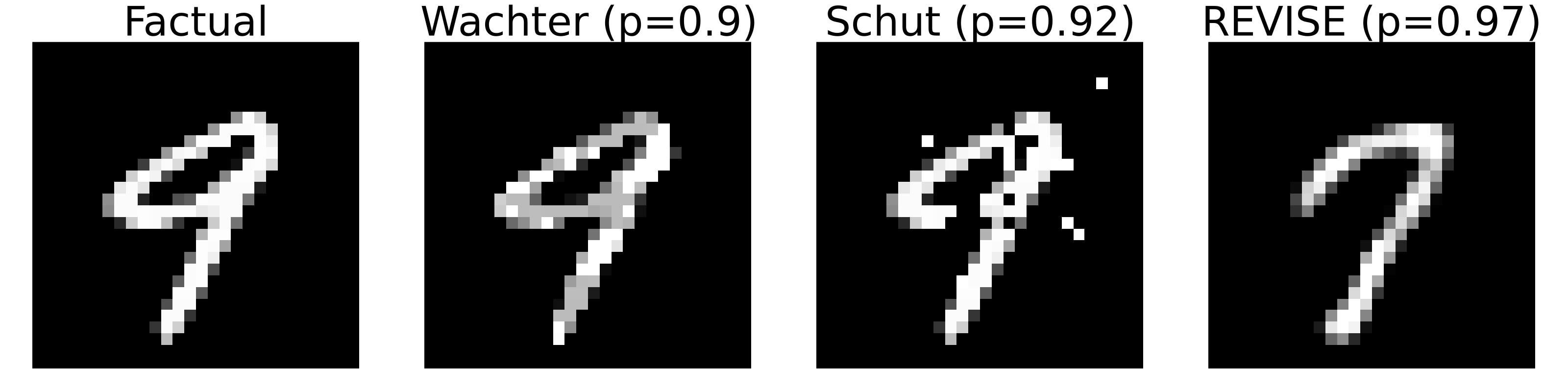
Since Wachter is only concerned with closeness, the generated counterfactual is almost indistinguishable from the factual. Schut expects a well-calibrated model that can generate predictive uncertainty estimates. Since this is not the case, the generated counterfactual looks like an adversarial example. Finally, the counterfactual generated by REVISE looks much more plausible than the other two. But is it also more faithful to the behavior of our MNIST classifier? That is much less clear because the surrogate used by REVISE introduces friction: explanations no longer depend exclusively on the black-box model itself.
So which of the counterfactuals most faithfully explains the behavior of our image classifier? Fidelity cannot help us to make that judgement, because all of these counterfactuals have full fidelity. Thus, fidelity is an insufficient evaluation metric to assess the faithfulness of CE.
4.4 Faithful first, Plausible second
Considering the limitations of fidelity as demonstrated in the previous section, analogous to Definition 4.1, we introduce a new notion of faithfulness in the context of CE:
Definition 4.2 (Faithful Counterfactuals) Let \(\mathcal{X}_{\theta}|\mathbf{y}^+ = p_{\theta}(\mathbf{x}|\mathbf{y}^+)\) denote the conditional distribution of \(\mathbf{x}\) in the target class \(\mathbf{y}^+\), where \(\theta\) denotes the parameters of model \(M_{\theta}\). Then for \(\mathbf{x}^{\prime}\) to be considered a faithful counterfactual, we need: \(\mathbf{x}^{\prime} \sim \mathcal{X}_{\theta}|\mathbf{y}^+\).
In doing this, we merge in and nuance the concept of plausibility (Definition 4.1) where the notion of ‘consistent with the data’ becomes ‘consistent with what the model has learned about the data’.
4.4.1 Quantifying the Model’s Generative Property
To assess counterfactuals with respect to Definition 4.2, we need a way to quantify the posterior conditional distribution \(p_{\theta}(\mathbf{x}|\mathbf{y}^+)\). To this end, we draw on ideas from energy-based modelling (EBM), a subdomain of machine learning that is concerned with generative or hybrid modelling (Grathwohl et al. 2020; Du and Mordatch 2020). In particular, note that if we fix \(\mathbf{y}\) to our target value \(\mathbf{y}^+\), we can conditionally draw from \(p_{\theta}(\mathbf{x}|\mathbf{y}^+)\) by randomly initializing \(\mathbf{x}_0\) and then using Stochastic Gradient Langevin Dynamics (SGLD) as follows,
\[ \begin{aligned} \mathbf{x}_{j+1} &\leftarrow \mathbf{x}_j - \frac{\epsilon_j^2}{2} \mathcal{E}_{\theta}(\mathbf{x}_j|\mathbf{y}^+) + \epsilon_j \mathbf{r}_j, && j=1,...,J \end{aligned} \tag{4.2}\]
where \(\mathbf{r}_j \sim \mathcal{N}(\mathbf{0},\mathbf{I})\) is the stochastic term and the step-size \(\epsilon_j\) is typically polynomially decayed (Welling and Teh 2011). The term \(\mathcal{E}_{\theta}(\mathbf{x}_j|\mathbf{y}^+)\) denotes the model energy conditioned on the target class label \(\mathbf{y}^+\) which we specify as the negative logit corresponding to \(\mathbf{y}^{+}\). To allow for faster sampling, we follow the common practice of choosing the step-size \(\epsilon_j\) and the standard deviation of \(\mathbf{r}_j\) separately. While \(\mathbf{x}_J\) is only guaranteed to distribute as \(p_{\theta}(\mathbf{x}|\mathbf{y}^{+})\) if \(\epsilon \rightarrow 0\) and \(J \rightarrow \infty\), the bias introduced for a small finite \(\epsilon\) is negligible in practice (Murphy 2023).
Generating multiple samples using SGLD thus yields an empirical distribution \(\widehat{\mathbf{X}}_{\theta,\mathbf{y}^+}\) that approximates what the model has learned about the input data. While in the context of EBM, this is usually done during training, we propose to repurpose this approach during inference in order to evaluate the faithfulness of model explanations. The appendix provides additional implementation details for any tasks related to energy-based modelling1.
4.4.2 Quantifying the Model’s Predictive Uncertainty
Faithful counterfactuals can be expected to also be plausible if the learned conditional distribution \(\mathcal{X}_{\theta}|\mathbf{y}^+\) (Definition 4.2) is close to the true conditional distribution \(\mathcal{X}|\mathbf{y}^+\) (Definition 4.1). We can further improve the plausibility of counterfactuals without the need for surrogate models that may interfere with faithfulness by minimizing predictive uncertainty (Schut et al. 2021). Unfortunately, this idea relies on the assumption that the model itself provides predictive uncertainty estimates, which may be too restrictive in practice.
To relax this assumption, we use conformal prediction (CP), an approach to predictive uncertainty quantification that has recently gained popularity (Angelopoulos and Bates 2022; Manokhin 2022). Crucially for our intended application, CP is model-agnostic and can be applied during inference without placing any restrictions on model training. It works under the premise of turning heuristic notions of uncertainty into rigorous estimates by repeatedly sifting through the training data or a dedicated calibration dataset. Calibration data is used to compute so-called nonconformity scores: \(\mathcal{S}=\{s(\mathbf{x}_i,\mathbf{y}_i)\}_{i \in \mathcal{D}_{\text{cal}}}\) where \(s: (\mathcal{X},\mathcal{Y}) \mapsto \mathbb{R}\) is referred to as score function (see appendix for details).
Conformal classifiers produce prediction sets for individual inputs that include all output labels that can be reasonably attributed to the input. These sets are formed as follows,
\[ \begin{aligned} C_{\theta}(\mathbf{x}_i;\alpha)=\{\mathbf{y}: s(\mathbf{x}_i,\mathbf{y}) \le \hat{q}\} \end{aligned} \tag{4.3}\]
where \(\hat{q}\) denotes the \((1-\alpha)\)-quantile of \(\mathcal{S}\) and \(\alpha\) is a predetermined error rate. These sets tend to be larger for inputs that do not conform with the training data and are characterized by high predictive uncertainty. To leverage this notion of predictive uncertainty in the context of gradient-based counterfactual search, we use a smooth set size penalty introduced by Stutz et al. (2022):
\[ \begin{aligned} \Omega(C_{\theta}(\mathbf{x};\alpha))&=\max \left(0, \sum_{\mathbf{y}\in\mathcal{Y}}C_{\theta,\mathbf{y}}(\mathbf{x}_i;\alpha) - \kappa \right) \end{aligned} \tag{4.4}\]
Here, \(\kappa \in \{0,1\}\) is a hyper-parameter and \(C_{\theta,\mathbf{y}}(\mathbf{x}_i;\alpha)\) can be interpreted as the probability of label \(\mathbf{y}\) being included in the prediction set (see appendix for details). In order to compute this penalty for any black-box model, we merely need to perform a single calibration pass through a holdout set \(\mathcal{D}_{\text{cal}}\). Arguably, data is typically abundant and in most applications, practitioners tend to hold out a test data set anyway. Consequently, CP removes the restriction on the family of predictive models, at the small cost of reserving a subset of the available data for calibration. This particular case of conformal prediction is referred to as split conformal prediction (SCP) as it involves splitting the training data into a proper training dataset and a calibration dataset.
4.4.3 Evaluating Plausibility and Faithfulness
The parallels between our definitions of plausibility and faithfulness imply that we can also use similar evaluation metrics in both cases. Since existing work has focused heavily on plausibility, it offers a useful starting point. In particular, Guidotti (2022) have proposed an implausibility metric that measures the distance of the counterfactual from its nearest neighbor in the target class. As this distance is reduced, counterfactuals get more plausible under the assumption that the nearest neighbor itself is plausible in the sense of Definition 4.1. In this work, we use the following adapted implausibility metric,
\[ \begin{aligned} \text{impl}(\mathbf{x}^{\prime},\mathbf{X}_{\mathbf{y}^+}) = \frac{1}{\lvert\mathbf{X}_{\mathbf{y}^+}\rvert} \sum_{\mathbf{x} \in \mathbf{X}_{\mathbf{y}^+}} \text{dist}(\mathbf{x}^{\prime},\mathbf{x}) \end{aligned} \tag{4.5}\]
where \(\mathbf{x}^{\prime}\) denotes the counterfactual and \(\mathbf{X}_{\mathbf{y}^+}\) is a subsample of the training data in the target class \(\mathbf{y}^+\). By averaging over multiple samples in this manner, we avoid the risk that the nearest neighbor of \(\mathbf{x}^{\prime}\) itself is not plausible according to Definition 4.1 (e.g. an outlier).
Equation 4.5 gives rise to a similar evaluation metric for unfaithfulness. We swap out the subsample of observed individuals in the target class for the set of samples generated through SGLD (\(\widehat{\mathbf{X}}_{\theta,\mathbf{y}^+}\)):
\[ \begin{aligned} \text{unfaith}(\mathbf{x}^{\prime},\widehat{\mathbf{X}}_{\theta,\mathbf{y}^+}) = \frac{1}{\lvert \widehat{\mathbf{X}}_{\theta,\mathbf{y}^+} \rvert} \sum_{\mathbf{x} \in \widehat{\mathbf{X}}_{\theta,\mathbf{y}^+}} \text{dist}(\mathbf{x}^{\prime},\mathbf{x}) \end{aligned} \tag{4.6}\]
Our default choice for the \(\text{dist}(\cdot)\) function in both cases is the Euclidean Norm. Depending on the type of input data other choices may be more adequate (see Section 4.6.1).
4.5 Energy-Constrained Conformal Counterfactuals
Given our proposed notion of faithfulness, we now describe ECCCo, our proposed framework for generating Energy-Constrained Conformal Counterfactuals. It is based on the premise that counterfactuals should first and foremost be faithful. Plausibility, as a secondary concern, is then still attainable to the degree that the black-box model itself has learned plausible explanations for the underlying data.
We begin by substituting the loss function in Equation 5.1,
\[ \begin{aligned} \min_{\mathbf{Z}^\prime \in \mathcal{Z}^L} \{ {L_{\text{JEM}}(f(\mathbf{Z}^\prime);M_{\theta},\mathbf{y}^+)}+ \lambda {\text{cost}(f(\mathbf{Z}^\prime)) } \} \end{aligned} \tag{4.7}\]
where \(L_{\text{JEM}}(f(\mathbf{Z}^\prime);M_{\theta},\mathbf{y}^+)\) is a hybrid loss function used in joint-energy modelling evaluated at a given counterfactual state for a given model and target outcome:
\[ \begin{aligned} L_{\text{JEM}}(f(\mathbf{Z}^\prime); \cdot) = L_{\text{clf}}(f(\mathbf{Z}^\prime); \cdot) + L_{\text{gen}}(f(\mathbf{Z}^\prime); \cdot) \end{aligned} \tag{4.8}\]
The first term, \(L_{\text{clf}}\), is any standard classification loss function such as cross-entropy loss. The second term, \(L_{\text{gen}}\), is used to measure loss with respect to the generative task2. In the context of joint-energy training, \(L_{\text{gen}}\) induces changes in model parameters \(\theta\) that decrease the energy of observed samples and increase the energy of samples generated through SGLD (Du and Mordatch 2020).
The key observation in our context is that we can rely solely on decreasing the energy of the counterfactual itself. This is sufficient to capture the generative property of the underlying model since it is implicitly captured by its parameters \(\theta\). Importantly, this means that we do not need to generate conditional samples through SGLD during our counterfactual search at all (see appendix for details).
This observation leads to the following simple objective function for ECCCo:
\[ \begin{aligned} & \min_{\mathbf{Z}^\prime \in \mathcal{Z}^L} \{ {L_{\text{clf}}(f(\mathbf{Z}^\prime);M_{\theta},\mathbf{y}^+)}+ \lambda_1 {\text{cost}(f(\mathbf{Z}^\prime)) } \\ &+ \lambda_2 \mathcal{E}_{\theta}(f(\mathbf{Z}^\prime)|\mathbf{y}^+) + \lambda_3 \Omega(C_{\theta}(f(\mathbf{Z}^\prime);\alpha)) \} \end{aligned} \tag{4.9}\]
The first penalty term involving \(\lambda_1\) induces closeness like in Wachter, Mittelstadt, and Russell (2017). The second penalty term involving \(\lambda_2\) induces faithfulness by constraining the energy of the generated counterfactual. The third and final penalty term involving \(\lambda_3\) ensures that the generated counterfactual is associated with low predictive uncertainty. To tune these hyperparameters we have relied on grid search.
Concerning feature autoencoding (\(f: \mathcal{Z} \mapsto \mathcal{X}\)), ECCCo does not rely on latent space search to achieve its primary objective of faithfulness. By default, we choose \(f(\cdot)\) to be the identity function as in Wachter. This is generally also enough to achieve plausibility, provided the model has learned plausible explanations for the data. In some cases, plausibility can be improved further by mapping counterfactuals to a lower-dimensional latent space. In the following, we refer to this approach as ECCCo+: that is, ECCCo plus dimensionality reduction.
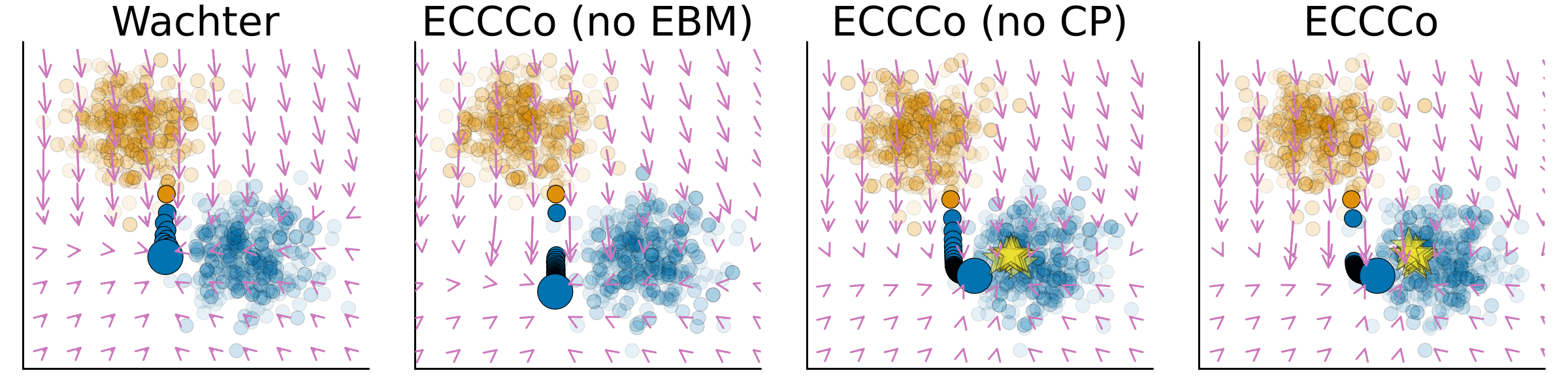
Figure 5.1 illustrates how the different components in Equation 4.9 affect the counterfactual search for a synthetic dataset. The underlying classifier is a Joint Energy Model (JEM) that was trained to predict the output class (blue or orange) and generate class-conditional samples (Grathwohl et al. 2020). We have used four different generator flavors to produce a counterfactual in the blue class for a sample from the orange class: Wachter, which only uses the first penalty (\(\lambda_2=\lambda_3=0\)); ECCCo (no EBM), which does not constrain energy (\(\lambda_2=0\)); ECCCo (no CP), which involves no set size penalty (\(\lambda_3=0\)); and, finally, ECCCo, which involves all penalties defined in Equation 4.9. Arrows indicate (negative) gradients with respect to the objective function at different points in the feature space.
While Wachter generates a valid counterfactual, it ends up close to the original starting point consistent with its objective. ECCCo (no EBM) avoids regions of high predictive uncertainty near the decision boundary, but the outcome is still not plausible. The counterfactual produced by ECCCo (no CP) is energy-constrained. Since the JEM has learned the conditional input distribution reasonably well in this case, the counterfactual is both faithful and plausible. Finally, the outcome for ECCCo looks similar, but the additional smooth set size penalty leads to somewhat faster convergence.
4.6 Empirical Analysis
Our goal in this section is to shed light on the following research questions:
Research Question 4.1 (Faithfulness) To what extent are counterfactuals generated by ECCCo more faithful than those produced by state-of-the-art generators?
Research Question 4.2 (Balancing Desiderata) Compared to state-of-the-art generators, how does ECCCo balance the two key objectives of faithfulness and plausibility?
The second question is motivated by the intuition that faithfulness and plausibility should coincide for models that have learned plausible explanations of the data.
4.6.1 Experimental Setup
To assess and benchmark the performance of our proposed generator against the state of the art, we generate multiple counterfactuals for different models and datasets. In particular, we compare ECCCo and its variants to the following counterfactual generators that were introduced above: firstly, Schut, which works under the premise of minimizing predictive uncertainty; secondly, REVISE, which is state-of-the-art (SOTA) with respect to plausibility; and, finally, Wachter, which serves as our baseline. In the case of ECCCo+, we use principal component analysis (PCA) for dimensionality reduction: the latent space \(\mathcal{Z}\) is spanned by the first \(n_z\) principal components where we choose \(n_z\) to be equal to the latent dimension of the VAE used by REVISE.
For the predictive modelling tasks, we use multi-layer perceptrons (MLP), deep ensembles, joint energy models (JEM) and convolutional neural networks (LeNet-5 CNN (LeCun et al. 1998)). Both joint-energy modelling and ensembling have been associated with improved generative properties and adversarial robustness (Grathwohl et al. 2020; Lakshminarayanan, Pritzel, and Blundell 2017), so we expect this to be positively correlated with the plausibility of ECCCo. To account for stochasticity, we generate many counterfactuals for each target class, generator, model and dataset over multiple runs.
We perform benchmarks on eight datasets from different domains. From the credit and finance domain we include three tabular datasets: Give Me Some Credit (GMSC) (Kaggle 2011), German Credit (Hoffman 1994) and California Housing (Pace and Barry 1997). All of these are commonly used in the related literature (Karimi et al. 2021; Altmeyer et al. 2023; Pawelczyk et al. 2021). Following related literature (Schut et al. 2021; Dhurandhar et al. 2018) we also include two image datasets: MNIST (LeCun et al. 1998) and Fashion MNIST (Xiao, Rasul, and Vollgraf 2017).
Full details concerning model training as well as detailed descriptions and results for all datasets can be found in the appendix. In the following, we will focus on the most relevant results highlighted in Table 4.1 and Table 4.2. The tables show sample averages along with standard deviations across multiple runs for our key evaluation metrics for the California Housing and GMSC datasets (Table 4.1) and the MNIST dataset (Table 4.2). For each metric, the best outcomes are highlighted in bold. Asterisks indicate that the given value is more than one (*) or two (**) standard deviations away from the baseline (Wachter). For the tabular datasets, we use the default Euclidean distance to measure unfaithfulness and implausibility as defined in Equation 4.6 and Equation 4.5, respectively. The third metric presented in Table 4.1 quantifies the predictive uncertainty of the counterfactual as measured by Equation 4.4. For the vision datasets, we rely on measuring the structural dissimilarity between images for our unfaithfulness and implausibility metrics (Wang, Simoncelli, and Bovik 2003).
4.6.2 Faithfulness
Overall, we find strong empirical evidence suggesting that ECCCo consistently achieves state-of-the-art faithfulness. Across all models and datasets highlighted here, different variations of ECCCo consistently outperform other generators with respect to faithfulness, in many cases substantially. This pattern is mostly robust across all other datasets.
In particular, we note that the best results are generally obtained when using the full ECCCo objective (Equation 4.9). In other words, constraining both energy and predictive uncertainty typically yields the most faithful counterfactuals. We expected the former to play a more significant role in this context and that is typically what we find across all datasets. The results in Table 4.1 indicate that faithfulness can be improved substantially by relying solely on the energy constraint (ECCCo (no CP)). In most cases, however, the full objective yields the most faithful counterfactuals. This indicates that predictive uncertainty minimization plays an important role in achieving faithfulness.
We also generally find that latent space search does not impede faithfulness for ECCCo. In most cases ECCCo+ is either on par with ECCCo or even outperforms it. There are some notable exceptions though. Cases in which ECCCo achieves substantially better faithfulness without latent space search tend to involve more vulnerable models like the simple MLP for MNIST in Table 4.2. We explain this finding as follows: even though dimensionality reduction through PCA in the case of ECCCo+ can be considered a relatively mild form of intervention, the first \(n_z\) principal components fail to capture some of the variation in the data. More vulnerable models may be particularly sensitive to this residual variation in the data.
Consistent with this finding, we also observe that REVISE ranks higher for faithfulness, if the model itself has learned more plausible representations of the underlying data: REVISE generates more faithful counterfactuals than the baseline for the JEM Ensemble in Table 4.1 and the LeNet-5 CNN in Table 4.2. This demonstrates that the two desiderata—faithfulness and plausibility—are not mutually exclusive.
4.6.3 Balancing Desiderata
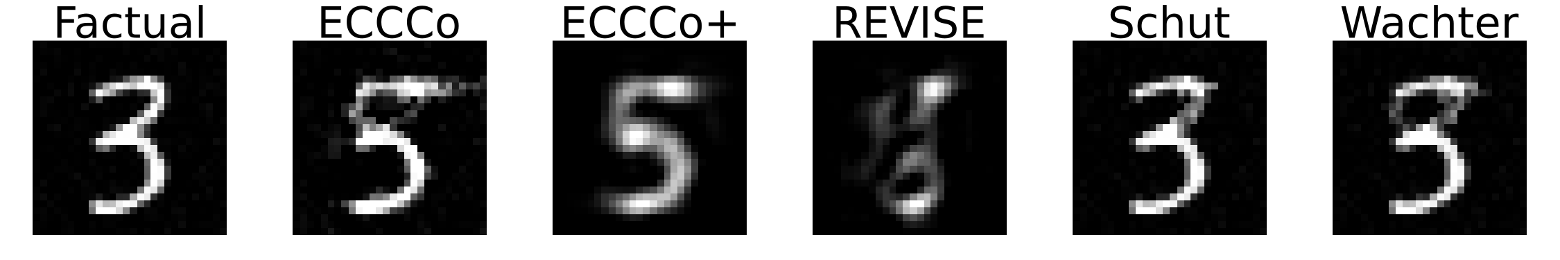
Overall, we find strong empirical evidence suggesting that ECCCo can achieve near state-of-the-art plausibility without sacrificing faithfulness. Figure 4.3 shows one such example taken from the MNIST benchmark where the objective is to turn the factual ‘three’ (far left) into a ‘five’. The underlying model is a LeNet-5 CNN. The different images show the counterfactuals produced by the generators, of which all but the one produced by Schut are valid. Both variations of ECCCo produce plausible counterfactuals.
Looking at the benchmark results presented in Table 4.1 and Table 4.2 we firstly note that although REVISE generally performs best, ECCCo and in particular ECCCo+ often approach SOTA performance. Upon visual inspection of the generated images we actually find that ECCCo+ performs much better than REVISE (see appendix). Zooming in on the details we observe that ECCCo and its variations do particularly well, whenever the underlying model has been explicitly trained to learn plausible representations of the data. For both tabular datasets in Table 4.1, ECCCo improves plausibility substantially compared to the baseline. This broad pattern is mostly consistent for all other datasets, although there are notable exceptions for which ECCCo takes the lead on both plausibility and faithfulness.
While we maintain that generally speaking plausibility should hinge on the quality of the model, our results also indicate that it is possible to balance faithfulness and plausibility if needed: ECCCo+ generally outperforms other variants of ECCCo in this context, occasionally at the small cost of slightly reduced faithfulness. For the vision datasets especially, we find that ECCCo+ is consistently second only to REVISE for all models and regularly substantially better than the baseline. Looking at the California Housing data, latent space search markedly improves plausibility without sacrificing faithfulness: for the JEM Ensemble, ECCCo+ performs substantially better than the baseline and only marginally worse than REVISE. Importantly, ECCCo+ does not attain plausibility at all costs: for the MLP Ensemble, plausibility is still very low, but this seems to faithfully represent what the model has learned.
We conclude from the findings presented thus far that ECCCo enables us to reconcile the objectives of faithfulness and plausibility. It produces plausible counterfactuals if and only if the model itself has learned plausible explanations for the data. It thus avoids the risk of generating plausible but potentially misleading explanations for models that are highly susceptible to implausible explanations.
4.6.4 Additional Desiderata
While we have deliberately focused on our key metrics of interest so far, it is worth briefly considering other common desiderata for counterfactuals. With reference to the right-most columns for each dataset in Table 4.1, we firstly note that ECCCo typically reduces predictive uncertainty as intended. Consistent with its design, Schut performs well on this metric even though it does not explicitly address uncertainty as measured by conformal prediction set sizes.
Another commonly discussed desideratum is closeness (Wachter, Mittelstadt, and Russell 2017): counterfactuals that are closer to their factuals are associated with smaller costs to individuals in the context of algorithmic recourse. As evident from the additional tables in the appendix, the closeness desideratum tends to be negatively correlated with plausibility and faithfulness. Consequently, both REVISE and ECCCo generally yield more costly counterfactuals than the baseline. Nonetheless, ECCCo does not seem to stretch costs unnecessarily: in Figure 4.3 useful parts of the factual ‘three’ are clearly retained.
4.7 Limitations
Despite having taken considerable measures to study our methodology carefully, limitations can still be identified.
Firstly, we recognize that our proposed distance-based evaluation metrics for plausibility and faithfulness may not be universally applicable to all types of data. In any case, they depend on choosing a distance metric on a case-by-case basis, as we have done in this work. Arguably, commonly used metrics for measuring other desiderata such as closeness suffer from the same pitfall. We therefore think that future work on counterfactual explanations could benefit from defining universal evaluation metrics.
Relatedly, we note that our proposed metric for measuring faithfulness depends on the availability of samples generated through SGLD, which in turn requires gradient access for models. This means it cannot be used to evaluate non-differentiable classifiers. Consequently, we also have not applied ECCCo to some machine learning models commonly used for classification such as decision trees. Since ECCCo itself does not rely on SGLD, its defining penalty functions are indeed applicable to gradient-free counterfactual generators. This is an interesting avenue for future research.
Next, common challenges associated with energy-based modelling including sensitivity to scale, training instabilities and sensitivity to hyperparameters also apply to ECCCo to some extent. In grid searches for optimal hyperparameters, we have noticed that unless properly regularized, ECCCo is sometimes prone to overshoot for the energy constraint.
Finally, while we have used ablation to understand the roles of the different components of ECCCo, the scope of this work has prevented us from investigating the role of conformal prediction in this context more thoroughly. We have exclusively relied on split conformal prediction and have used fixed values for the predetermined error rate and other hyperparameters. Future work could benefit from more extensive ablation studies that tune hyperparameters and investigate different approaches to conformal prediction.
4.8 Conclusion
This work leverages ideas from energy-based modelling and conformal prediction in the context of counterfactual explanations. We have proposed a new way to generate counterfactuals that are maximally faithful to the black-box model they aim to explain. Our proposed generator, ECCCo, produces plausible counterfactuals iff the black-box model itself has learned realistic explanations for the data, which we have demonstrated through rigorous empirical analysis. This should enable researchers and practitioners to use counterfactuals in order to discern trustworthy models from unreliable ones. While the scope of this work limits its generalizability, we believe that ECCCo offers a solid base for future work on faithful counterfactual explanations.
4.9 Acknowledgements
Some of the members of TU Delft were partially funded by ICAI AI for Fintech Research, an ING—TU Delft collaboration.
Research reported in this work was partially or completely facilitated by computational resources and support of the DelftBlue ((DHPC) 2022) and the Delft AI Cluster (DAIC: https://doc.daic.tudelft.nl/) at TU Delft. Detailed information about the utilized computing resources can be found in the appendix. The authors would like to thank Azza Ahmed, in particular, for her tremendous help with running Julia jobs on the cluster. The work remains the sole responsibility of the authors.
We would also like to express our gratitude to the group of students who have recently contributed to the development of CounterfactualExplanations.jl (Chapter 2), the Julia package that was used for this analysis: Rauno Arike, Simon Kasdorp, Lauri Kesküll, Mariusz Kicior, Vincent Pikand.
All code used for the analysis in this paper can be found here: https://github.com/pat-alt/ECCCo.jl.