5 Counterfactual Training: Teaching Models Plausible and Actionable Explanations
We propose a novel training regime termed counterfactual training that leverages counterfactual explanations to increase the explanatory capacity of models. Counterfactual explanations have emerged as a popular post-hoc explanation method for opaque machine learning models: they inform how factual inputs would need to change in order for a model to produce some desired output. To be useful in real-world decision-making systems, counterfactuals should be plausible with respect to the underlying data and actionable with respect to the feature mutability constraints. Much existing research has therefore focused on developing post-hoc methods to generate counterfactuals that meet these desiderata. In this work, we instead hold models directly accountable for the desired end goal: counterfactual training employs counterfactuals during the training phase to minimize the divergence between learned representations and plausible, actionable explanations. We demonstrate empirically and theoretically that our proposed method facilitates training models that deliver inherently desirable counterfactual explanations and additionally exhibit improved adversarial robustness.
Counterfactual Training, Counterfactual Explanations, Algorithmic Recourse, Explainable AI, Adversarial Robustness
5.1 Introduction
Today’s prominence of artificial intelligence (AI) has largely been driven by the success of representation learning with high degrees of freedom: instead of relying on features and rules hand-crafted by humans, modern machine learning (ML) models are tasked with learning highly complex representations directly from the data, guided by narrow objectives such as predictive accuracy (Goodfellow, Bengio, and Courville 2016). These models tend to be so complex that humans cannot easily interpret their decision logic.
Counterfactual explanations (CE) have become a key part of the broader explainable AI (XAI) toolkit (Molnar 2022) that can be applied to make sense of this complexity. They prescribe minimal changes for factual inputs that, if implemented, would prompt some fitted model to produce an alternative, more desirable output (Wachter, Mittelstadt, and Russell 2017). This is useful and necessary to not only understand how opaque models make their predictions, but also to provide algorithmic recourse to individuals subjected to them: a retail bank, for example, could use CE to provide meaningful feedback to unsuccessful loan applicants that were rejected based on an opaque automated decision-making (ADM) system (Figure 5.1).
For such feedback to be meaningful, counterfactual explanations need to fulfill certain desiderata (Verma et al. 2022; Karimi et al. 2021)—they should be faithful to the model (Altmeyer et al. 2024), plausible (Joshi et al. 2019), and actionable (Ustun, Spangher, and Liu 2019). Plausibility is typically understood as counterfactuals being in-domain: unsuccessful loan applicants that implement the provided recourse should end up with credit profiles that are genuinely similar to that of individuals who have successfully repaid their loans in the past. Actionable explanations further comply with practical constraints: a young, unsuccessful loan applicant cannot increase their age in an instant.
Existing state-of-the-art (SOTA) approaches in the field have largely focused on designing model-agnostic CE methods that identify subsets of counterfactuals, which comply with specific desiderata. This is problematic because the narrow focus on any specific desideratum can adversely affect others: it is possible, for example, to generate plausible counterfactuals for models that are also highly vulnerable to implausible, possibly adversarial counterfactuals (Altmeyer et al. 2024). Indeed, existing approaches generally fail to guarantee that the representations learned by a model are compatible with truly meaningful explanations.
In this work, we propose an approach to bridge this gap, embracing the paradigm that models—as opposed to explanation methods—should be held accountable for explanations that are plausible and actionable. While previous work has shown that at least plausibility can be indirectly achieved through existing techniques aimed at models’ generative capacity, generalization and robustness (Altmeyer et al. 2024; Augustin, Meinke, and Hein 2020; Schut et al. 2021), we directly incorporate both plausibility and actionability in the training objective of models to improve their overall explanatory capacity.
Specifically, we introduce counterfactual training (CT): a novel training regime that leverages counterfactual explanations on-the-fly to ensure that differentiable models learn plausible and actionable explanations for the underlying data, while at the same time being more robust to adversarial examples (AE). Figure 5.1 illustrates the outcomes of CT compared to a conventionally trained model. First, in panel (a), faithful and valid counterfactuals end up near the decision boundary forming a clearly distinguishable cluster in the target class (orange). In panel (b), CT is applied to the same underlying linear classifier architecture resulting in much more plausible counterfactuals. In panel (c), the classifier is again trained conventionally and we have introduced a mutability constraint on the age feature at test time—counterfactuals are valid but the classifier is roughly equally sensitive to both features. By contrast, the decision boundary in panel (d) has tilted, making the model trained with CT relatively less sensitive to the immutable age feature. To achieve these outcomes, CT draws inspiration from the literature on contrastive and robust learning: we contrast faithful CEs with ground-truth data while protecting immutable features, and capitalize on methodological links between CE and AE by penalizing the model’s adversarial loss on interim (nascent) counterfactuals. To the best of our knowledge, CT represents the first venture in this direction with promising empirical and theoretical results.
The remainder of this manuscript is structured as follows. Section 5.2 presents related work, focusing on the links to contrastive and robust learning. Then follow our two principal contributions. In Section 5.3, we introduce our methodological framework and show theoretically that it can be employed to respect global actionability constraints. In our experiments (Section 5.4), we find that thanks to counterfactual training, (1) the implausibility of CEs decreases by up to 90%; (2) the cost of reaching valid counterfactuals with protected features decreases by 19% on average; and (3) models’ adversarial robustness improves across the board. Finally, we discuss open challenges in Section 5.5 and conclude in Section 5.6.

5.2 Related Literature
To make the desiderata for CT more concrete, we follow previous work, tying the explanatory capacity of models to the quality of CEs that can be generated for them (Altmeyer et al. 2024; Augustin, Meinke, and Hein 2020).
5.2.1 Explanatory Capacity and Contrastive Learning
A closely related work shows that model averaging and, in particular, contrastive model objectives can produce models that have a higher explanatory capacity, and hence ones that are more trustworthy (Altmeyer et al. 2024). The authors propose a way to generate counterfactuals that are maximally faithful in that they are consistent with what models have learned about the underlying data. Formally, they rely on tools from energy-based modelling (Teh et al. 2003) to minimize the contrastive divergence between the distribution of counterfactuals and the conditional posterior over inputs learned by a model. Their algorithm, ECCCo, yields plausible counterfactual explanations if and only if the underlying model has learned representations that align with them. The authors find that both deep ensembles (Lakshminarayanan, Pritzel, and Blundell 2017) and joint energy-based models (JEMs) (Grathwohl et al. 2020), a form of contrastive learning, do well in this regard.
It helps to look at these findings through the lens of representation learning with high degrees of freedom. Deep ensembles are approximate Bayesian model averages, which are particularly effective when models are underspecified by the available data (Wilson 2020). Averaging across solutions mitigates the risk of overrelying on a single locally optimal representation that corresponds to semantically meaningless explanations. Likewise, it has been shown that generating plausible (“interpretable”) CEs is almost trivial for deep ensembles that have undergone adversarial training (Schut et al. 2021). The case for JEMs is even clearer: they optimize a hybrid objective that induces both high predictive performance and strong generative capacity (Grathwohl et al. 2020), resembling the idea of aligning models with plausible explanations. This was an inspiration for CT.
5.2.2 Explanatory Capacity and Robust Learning
Prior work has shown that counterfactual explanations tend to be more meaningful (“explainable”) if the underlying model is more robust to adversarial examples (Augustin, Meinke, and Hein 2020). Once again, we can make intuitive sense of this finding if we look at adversarial training (AT) through the lens of representation learning with high degrees of freedom: highly complex and flexible models may learn representations that make them sensitive to implausible or even adversarial examples (Szegedy et al. 2014). Thus, by inducing models to “unlearn” susceptibility to such examples, adversarial training can effectively remove implausible explanations from the solution space.
This interpretation of the link between explanatory capacity through counterfactuals on the one side, and robustness to adversarial examples on the other is backed by empirical evidence. Firstly, prior work has shown that using counterfactual images during classifier training improves model robustness (Sauer and Geiger 2021). Similarly, related work has shown that counterfactuals represent potentially useful training data in machine learning tasks, especially in supervised settings where inputs may be reasonably mapped to multiple outputs (Abbasnejad et al. 2020). The authors show that augmenting the training data of (image) classifiers can improve generalization performance. Finally, another related work has demonstrated that counterfactual pairs tend to exist in training data (Teney, Abbasnedjad, and Hengel 2020). Hence, the proposed approach aims to identify similar inputs with different annotations and ensure that the gradient of the classifier aligns with the vector between such pairs of inputs using a cosine distance loss function.
CEs have also been used to improve models in the natural language processing domain. A well-known paper in this domain has proposed Polyjuice (Wu et al. 2021), a general-purpose CE generator for language models. The authors demonstrate that the augmentation of training data with Polyjuice improves robustness in a number of tasks. Related work has introduced the Counterfactual Adversarial Training (CAT) framework (Luu and Inoue 2023), which aims to improve generalization and robustness of language models by generating counterfactuals for training samples that are subject to high predictive uncertainty.
There have also been several attempts at formalizing the relationship between counterfactual explanations and adversarial examples. Pointing to clear similarities in how CEs and AEs are generated, prior work makes the case for jointly studying the opaqueness and robustness problems in representation learning (Freiesleben 2022). Formally, the authors show that AEs can be seen as the subset of CEs for which misclassification is achieved (Freiesleben 2022). Similarly, others have shown that CEs and AEs are equivalent under certain conditions (Pawelczyk et al. 2022).
Two other works are closely related to ours in that they use counterfactuals during training with the explicit goal of affecting certain properties of the post-hoc counterfactual explanations. The first closely related work has proposed a way to train models that guarantee recourse to a positive target class with high probability (Ross, Lakkaraju, and Bastani 2024). The approach builds on adversarial training by explicitly inducing susceptibility to targeted AEs for the positive class. Additionally, the method allows for imposing a set of actionability constraints ex-ante. For example, users can specify that certain features are immutable. A second closely related work has introduced the first end-to-end training pipeline that includes CEs as part of the training procedure (Guo, Nguyen, and Yadav 2023); the CounterNet network architecture includes a predictor and a CE generator, where the parameters of the CE generator are learnable. Counterfactuals are generated during each training iteration and fed back to the predictor. In contrast, we impose no restrictions on the artificial neural network architecture at all.
5.3 Counterfactual Training
This section introduces the counterfactual training framework, applying ideas from contrastive and robust learning to counterfactual explanations. CT produces models whose learned representations align with plausible explanations that comply with user-defined actionability constraints.
Counterfactual explanations are typically generated by solving variations of the following optimization problem,
\[ \begin{aligned} \min_{\mathbf{x}^\prime \in \mathcal{X}^D} \left\{ {\text{yloss}(\mathbf{M}_\theta(\mathbf{x}^{\prime}),\mathbf{y}^+)}+ \lambda {\text{reg}(\mathbf{x}^{\prime}) } \right\} \end{aligned} \tag{5.1}\]
where \(\mathbf{M}_\theta: \mathcal{X} \mapsto \mathcal{Y}\) denotes a classifier, \(\mathbf{x}^{\prime}\) denotes the counterfactual with \(D\) features and \(\mathbf{y}^+\in\mathcal{Y}\) denotes some target class. The \(\text{yloss}(\cdot)\) function quantifies the discrepancy between current model predictions for \(\mathbf{x}^{\prime}\) and the target class (a conventional choice is cross-entropy). Finally, we use \(\text{reg}(\cdot)\) to denote any form of regularization used to induce certain properties on the counterfactual. The seminal CE paper, (Wachter, Mittelstadt, and Russell 2017), proposes regularizing the distance between counterfactuals and their original factual values to ensure that individuals seeking recourse through CE face minimal costs in terms of feature changes. Different variations of Equation 5.1 have been proposed in the literature to address many desiderata including the ones discussed above (faithfulness, plausibility and actionability). Much like in the seminal work (Wachter, Mittelstadt, and Russell 2017), most of these approaches rely on gradient descent to optimize Equation 5.1, and this holds true for all approaches tested in this work. We introduce them briefly in Section 5.4.1, but refer the reader to the supplementary appendix for details. In the following, we describe how counterfactuals are generated and used in CT.
5.3.1 Proposed Training Objective
The goal of CT is to improve the explanatory capacity of models by aligning the learned representations with faithful explanations that are plausible and actionable. For simplicity, we refer to models with high explanatory capacity as explainable in this manuscript. We define explainability as follows:
Definition 5.1 (Model Explainability) Let \(\mathbf{M}_\theta: \mathcal{X} \mapsto \mathcal{Y}\) denote a supervised classification model that maps from the \(D\)-dimensional input space \(\mathcal{X}\) to representations \(\phi(\mathbf{x};\theta)\) and finally to the \(K\)-dimensional output space \(\mathcal{Y}\). Let \(\mathbf{x}_0^\prime\) denote a factual input and assume that for any given input-output pair \(\{\mathbf{x}_0^\prime,\mathbf{y}\}_i\) there exists a counterfactual \(\mathbf{x}^{\prime} = \mathbf{x}_0^\prime + \Delta: \mathbf{M}_\theta(\mathbf{x}^{\prime}) = \mathbf{y}^{+} \neq \mathbf{y} = \mathbf{M}_\theta(\mathbf{x})\), where \(\arg\max_y{\mathbf{y}^{+}}=y^+\) is the index of the target class.
We say that \(\mathbf{M}_\theta\) has an explanatory capacity to the extent that faithfully generated, valid counterfactuals are also plausible and actionable. We define these properties as:
(Faithfulness) \(P(\mathbf{x}^\prime \in \mathcal{X}_\theta|\mathbf{y}^+) = 1 - \delta\), where \(\delta\) is some small value, and \(\mathcal{X}_\theta|\mathbf{y}^+\) is the conditional posterior distribution over inputs (adapted from (Altmeyer et al. 2024), Def. 4.1).
(Plausibility) \(P(\mathbf{x}^\prime \in \mathcal{X}|\mathbf{y}^+) = 1 - \delta\), where \(\delta\) is some small value, and \(\mathcal{X}|\mathbf{y}^+\) is the conditional distribution of inputs in the target class (adapted from (Altmeyer et al. 2024), Def. 2.1).
(Actionability) Perturbations \(\Delta\) may be subject to some actionability constraints.
Intuitively, plausible counterfactuals are consistent with the data, and faithful counterfactuals are consistent with what the model has learned about the input data. Actionability constraints in Definition 5.1 depend on the context in which \(\mathbf{M}_\theta\) is deployed (e.g., specified by end-users or model owners). We consider two types of actionability constraints: on the domain of features and on their mutability. The former naturally arise in automated decision-making systems whenever a feature can only take a specific range of values. For example, age is lower bounded by zero and upper bounded by the maximum human lifespan. Specifying such domain constraints can also help address training instabilities commonly associated with energy-based modelling (Grathwohl et al. 2020). The latter arise when a feature cannot be freely modified. Continuing the example, age of a person can only increase, but it may even be considered as an immutable feature: waiting many years for an improved outcome is hardly feasible for individuals affected by algorithmic decisions. We choose to only consider domain and mutability constraints for individual features \(x_d\) for \(d=1,...,D\). Of course, this is a simplification since feature values may correlate, e.g., higher age may be associated with higher level of completed education. We address this challenge in Section 5.5, where we also explain why we restrict this work to classification settings.
Let \(\mathbf{x}_t^\prime\) for \(t=0,...,T\) denote a counterfactual generated through gradient descent over \(T\) iterations as originally proposed (Wachter, Mittelstadt, and Russell 2017). CT adopts gradient-based CE search in training to generate on-the-fly model explanations \(\mathbf{x}^\prime\) for the training samples. We use the term nascent to denote interim counterfactuals \(\mathbf{x}_{\text{AE}}^\prime\) that have not yet converged. As we explain below, these nascent counterfactuals can be stored and repurposed as adversarial examples. Conversely, we consider counterfactuals \(\mathbf{x}_{\text{CE}}^\prime\) as mature explanations if they have converged within the \(T\) iterations by reaching a pre-specified threshold, \(\tau\), for the predicted probability of the target class: \(\mathcal{S}(\mathbf{M}_\theta(\mathbf{x}^\prime))[y^+] \geq \tau\), where \(\mathcal{S}\) is the softmax function.
Formally, we propose the following counterfactual training objective to train explainable (as in Definition 5.1) models,
\[ \begin{aligned} &\min_\theta \text{yloss}(\mathbf{M}_\theta(\mathbf{x}),\mathbf{y}) + \lambda_{\text{div}} \text{div}(\mathbf{x}^+,\mathbf{x}_{\text{CE}}^\prime,y^+;\theta) \\+ &\lambda_{\text{adv}} \text{advloss}(\mathbf{M}_\theta(\mathbf{x}_{\text{AE}}^\prime),\mathbf{y}_{\text{AE}}) + \lambda_{\text{reg}}\text{ridge}(\mathbf{x}^+,\mathbf{x}_{\text{CE}}^\prime,y;\theta) \end{aligned} \tag{5.2}\]
where \(\text{yloss}(\cdot)\) is any classification loss that induces discriminative performance (e.g., cross-entropy). The second and third terms are explained in detail in the following subsections. For now, they can be summarized as inducing explainability directly and indirectly by penalizing (1) the contrastive divergence, \(\text{div}(\cdot)\), between mature counterfactuals \(\mathbf{x}_{\text{CE}}^\prime\) and observed samples \(\mathbf{x}^+\in\mathcal{X}^+=\{\mathbf{x}:y=y^+\}\) in the target class \(y^+\), and (2) the adversarial loss, \(\text{advloss}(.)\), wrt. nascent counterfactuals \(\mathbf{x}_{\text{AE}}^\prime\) and their corresponding labels \(\mathbf{y}_{\text{AE}}\). Finally, \(\text{ridge}(\cdot)\) denotes a Ridge penalty (squared \(\ell_2\)-norm) that regularizes the magnitude of the energy terms involved in the contrastive divergence, \(\text{div}(\cdot)\), term (Du and Mordatch 2020):
\[ \frac{1}{n_{\text{CE}}} \sum_{i=1}^{n_{\text{CE}}} \left( \mathcal{E}_{\theta}(\mathbf{x^+},y^+)^2 + \mathcal{E}_{\theta}(\mathbf{x}_{\text{CE}}^\prime,y^+)^2 \right) \tag{5.3}\]
The trade-offs between these components are adjusted through penalties \(\lambda_{\text{div}}\), \(\lambda_{\text{adv}}\), and \(\lambda_{\text{reg}}\).
The full counterfactual training regime is sketched out in Algorithm 1. During each iteration, we do the following steps. Firstly, we randomly draw a subset of \(n_{\text{CE}} \leq n\) factuals \(\mathbf{x}_0^\prime\) from \(\mathbf{X}\) of size \(n\), for which we uniformly draw a target class \(y^+\) (ensuring that it does not coincide with the class currently predicted for \(\mathbf{x}_0^\prime\)) and a corresponding training sample from the target class, \(\mathbf{x}^+\sim \mathbf{X}^+=\{\mathbf{x} \in \mathbf{X}:y=y^+\}\). Secondly, we conduct the counterfactual search by solving (Equation 5.1) through gradient descent. Thirdly, we sample mini-batches \({(\mathbf{x}_i, \mathbf{y}_i)}_{i=1}^{n_b}\) from the training dataset \(\mathcal{D}=(\mathbf{X},\mathbf{Y})\) for conventional training and distribute the tuples composed of counterfactuals, their target labels and corresponding training samples, as well as adversarial examples and corresponding labels, \(({\mathbf{x}_{\text{CE}}^\prime}_i,{y^+}_i,{\mathbf{x}_{\text{AE}}^\prime}_i,{\mathbf{y}_{\text{AE}}}_i,{\mathbf{x}^+}_i)_{i=1}^{n_{\text{CE}}}\), across the mini-batches. Finally, we backpropagate through (Equation 5.2).
By limiting ourselves to a subset of \(n_{\text{CE}}\) counterfactuals, we reduce runtimes; this approach has previously been shown to improve efficiency in the context of adversarial training (Kurakin, Goodfellow, and Bengio 2017; Kaufmann et al. 2022). To improve runtimes even more, we choose to first generate counterfactuals and then distribute them across mini-batches to benefit from greater degrees of parallelization during the counterfactual search. Alternatively, it is possible to generate counterfactuals separately for each mini-batch.1
5.3.2 Directly Inducing Explainability: Contrastive Divergence
As observed in prior related work (Grathwohl et al. 2020), any classifier can be re-interpreted as a joint energy-based model that learns to discriminate output classes conditional on the observed (training) samples from \(p(\mathbf{x})\) and the generated samples from \(p_\theta(\mathbf{x})\). The authors show that JEMs can be trained to perform well at both tasks by directly maximizing the joint log-likelihood: \(\log p_\theta(\mathbf{x},\mathbf{y})=\log p_\theta(\mathbf{y}|\mathbf{x}) + \log p_\theta(\mathbf{x})\), where the first term can be optimized using cross-entropy as in Equation 5.2. To optimize \(\log p_\theta(\mathbf{x})\), they minimize the contrastive divergence between the observed samples from \(p(\mathbf{x})\) and samples generated from \(p_\theta(\mathbf{x})\).
To generate samples, the paper introducing JEMs (Grathwohl et al. 2020) suggests relying on Stochastic Gradient Langevin Dynamics (SGLD) with an uninformative prior for initialization but we depart from this methodology: we propose to leverage counterfactual explainers to generate counterfactuals of observed training samples. Specifically, we have:
\[ \text{div}(\mathbf{x}^+,\mathbf{x}_{\text{CE}}^\prime,y^+;\theta) = \mathcal{E}_\theta(\mathbf{x}^+,y^+) - \mathcal{E}_\theta(\mathbf{x}_{\text{CE}}^\prime,y^+) \tag{5.4}\]
where \(\mathcal{E}_\theta(\cdot)\) denotes the energy function defined as \(\mathcal{E}_\theta(\mathbf{x},y^+)=-\mathbf{M}_\theta(\mathbf{x})[y^+]\), with \(y^+\) denoting the index of the randomly drawn target class, \(y^+ \sim p(y)\). Conditional on the target class \(y^+\), \(\mathbf{x}_{\text{CE}}^\prime\) denotes a mature counterfactual for a randomly sampled factual from a non-target class generated with a gradient-based CE generator for up to \(T\) iterations. Intuitively, the gradient of Equation 5.4 decreases the energy of observed training samples (positive samples) while increasing the energy of counterfactuals (negative samples) (Du and Mordatch 2020). As the counterfactuals get more plausible (Definition 5.1) during training, these opposing effects gradually balance each other out (Lippe 2024).
Since the maturity of counterfactuals in terms of a probability threshold is often reached before \(T\), this form of sampling is not only more closely aligned with Definition 5.1., but can also speed up training times compared to SGLD. The departure from SGLD also allows us to tap into the vast repertoire of explainers that have been proposed in the literature to meet different desiderata. For example, many methods support domain and mutability constraints. In principle, any approach for generating CEs is viable, so long as it does not violate the faithfulness condition. Like JEMs (Murphy 2022), counterfactual training can be viewed as a form of contrastive representation learning.
5.3.3 Indirectly Inducing Explainability: Adversarial Robustness
Based on our analysis in Section 5.2, counterfactuals \(\mathbf{x}^\prime\) can be repurposed as additional training samples (Balashankar et al. 2023; Luu and Inoue 2023) or adversarial examples (Freiesleben 2022; Pawelczyk et al. 2022). This leaves some flexibility with regards to the choice for the \(\text{advloss}(\cdot)\) term in Equation 5.2. An intuitive functional form, but likely not the only sensible choice, is inspired by adversarial training:
\[ \begin{aligned} \text{advloss}(\mathbf{M}_\theta(\mathbf{x}_{\text{AE}}^\prime),\mathbf{y};\varepsilon)&=\text{yloss}(\mathbf{M}_\theta(\mathbf{x}_{t_\varepsilon}^\prime),\mathbf{y}) \\ t_\varepsilon &= \max_t \{t: ||\Delta_t||_\infty < \varepsilon\} \end{aligned} \tag{5.5}\]
Under this choice, we consider nascent counterfactuals \(\mathbf{x}_{\text{AE}}^\prime\) as AEs as long as the magnitude of the perturbation at time \(t\) (\(\Delta_t\)) to any single feature is at most \(\varepsilon\). The most strongly perturbed counterfactual \(\mathbf{x}_{t_\varepsilon}^\prime\) that still satisfies the condition is used as an adversarial example \(\mathbf{x}_{\text{AE}}^\prime\). This formalization is closely aligned with seminal work on adversarial machine learning (Szegedy et al. 2014), which defines an adversarial attack as an “imperceptible non-random perturbation”. Thus, we work with a different distinction between CE and AE than the one proposed in prior work (Freiesleben 2022), which considers misclassification as the distinguishing feature of adversarial examples. One of the key observations of our work is that we can leverage CEs during training and get AEs essentially for free to reap the benefits of adversarial training, leading to improved adversarial robustness and plausibility.
5.3.4 Encoding Actionability Constraints
Many existing counterfactual explainers support domain and mutability constraints. In fact, both types of constraints can be implemented for any explainer that relies on gradient descent in the feature space for optimization (Altmeyer, Deursen, and Liem 2023). In this context, domain constraints can be imposed by simply projecting counterfactuals back to the specified domain; if the previous gradient step resulted in updated feature values that were out-of-domain. Similarly, mutability constraints can be enforced by setting partial derivatives to zero to ensure that features are only perturbed in the allowed direction, if at all.
As actionability constraints are binding at test time, we must also impose them when generating \(\mathbf{x}^\prime\) during each training iteration to inform model representations. Through their effect on \(\mathbf{x}^\prime\), both types of constraints influence model outcomes via Equation 5.4. It is crucial that we avoid penalizing implausibility that arises from mutability constraints. For any mutability-constrained feature \(d\) this can be achieved by enforcing \(\mathbf{x}^+[d] - \mathbf{x}^\prime[d]:=0\), whenever perturbing \(\mathbf{x}^\prime[d]\) in the direction of \(\mathbf{x}^+[d]\) would violate mutability constraints defined for \(d\). Specifically, we set \(\mathbf{x}^+[d] := \mathbf{x}^\prime[d]\) if:
Feature \(d\) is strictly immutable in practice.
\(\mathbf{x}^+[d]>\mathbf{x}^\prime[d]\), but \(d\) can only be decreased in practice.
\(\mathbf{x}^+[d]<\mathbf{x}^\prime[d]\), but \(d\) can only be increased in practice.
From a Bayesian perspective, setting \(\mathbf{x}^+[d] := \mathbf{x}^\prime[d]\) can be understood as assuming a point mass prior for \(p(\mathbf{x}^+)\) with respect to feature \(d\), i.e., we can model this as absolute certainty that the value \(\mathbf{x}^+[d]\) remains the same as in the neighbor, \(\mathbf{x}^\prime[d]\), but it could be equivalently seen as masking changes to feature \(d\). Intuitively, we can think of this as ignoring implausibility costs of immutable features, which effectively forces the model to instead seek plausibility through the remaining features. This can be expected to produce a classifier with relatively lower sensitivity to immutable features, and the higher relative sensitivity to mutable features should make mutability-constrained recourse less costly (see Section 5.4). Under certain conditions, this result also holds theoretically (for the proof, see the supplementary appendix):
Proposition 5.1 (Protecting Immutable Features) Let \(f_\theta(\mathbf{x})=\mathcal{S}(\mathbf{M}_\theta(\mathbf{x}))=\mathcal{S}(\Theta\mathbf{x})\) denote a linear classifier with softmax activation \(\mathcal{S}\) where \(y\in\{1,...,K\}=\mathcal{K}\), \(\mathbf{x} \in \mathbb{R}^D\) and \(\Theta\) is the matrix of coefficients with \(\theta_{k,d}=\Theta[k,d]\) denoting the coefficient on feature \(d\) for class \(k\). Assume multivariate Gaussian class densities with a common diagonal covariance matrix \(\Sigma_k=\Sigma\) for all \(k \in \mathcal{K}\), then protecting an immutable feature from the contrastive divergence penalty will result in lower classifier sensitivity to that feature relative to the remaining features, provided that at least one of those is discriminative and mutable.
5.4 Experiments
We start by introducing the experimental setup, including performance metrics, datasets, algorithms, and explain our approach to evaluation in Section 5.4.1. Then, we address the research questions (RQ). Two questions relating to the principal goals of counterfactual training are presented in Section 5.4.2:
Research Question 5.1 To what extent does the CT objective in Equation 5.2 induce models to learn plausible explanations?
Research Question 5.2 To what extent does CT result in more favorable algorithmic recourse outcomes in the presence of actionability constraints
Next, in Section 5.4.3 we consider the performance of models trained with CT, focusing on their adversarial robustness but also commenting on the validity of generated CEs.
Research Question 5.3 To what extent does CT influence the adversarial robustness of trained models?
Finally, in Section 5.4.4 we perform an ablation of the CT objective and evaluate its sensitivity to hyperparameters:
Research Question 5.4 How does the CT objective depends on its individual components? (ablation)
Research Question 5.5 What are the effects of hyperparameter selection on counterfactual training?
5.4.1 Experimental Setup
Our focus is the improvement in explainability (Definition 5.1). Thus, we mainly look at the plausibility and cost of faithfully generated counterfactuals at test time, but several other metrics are covered in the supplementary appendix. To measure the cost, we follow the standard proxy of distances (\(\ell_1\)-norm) between factuals and counterfactuals. For plausibility, we assess how similar CEs are to observed samples in the target domain, \(\mathbf{X}^+\subset\mathcal{X}^+\). For the evaluation, we rely on the metric proposed in prior work (Altmeyer et al. 2024) with \(\ell_1\)-norm for distances,
\[ \text{IP}(\mathbf{x}^\prime,\mathbf{X}^+) = \frac{1}{\lvert\mathbf{X}^+\rvert}\sum_{\mathbf{x} \in \mathbf{X}^+} \text{dist}(\mathbf{x}^{\prime},\mathbf{x}) \tag{5.6}\]
and introduce a novel divergence-based adaptation,
\[ \text{IP}^*(\mathbf{X}^\prime,\mathbf{X}^+) = \text{MMD}(\mathbf{X}^\prime,\mathbf{X}^+) \tag{5.7}\]
where \(\mathbf{X}^\prime\) denotes a collection of counterfactuals and \(\text{MMD}(\cdot)\) is the unbiased estimate of the squared population maximum mean discrepancy (Gretton et al. 2012):
\[ \begin{aligned} \text{MMD}(\mathbf{X}^\prime,\mathbf{X}^+) &= \frac{1}{m(m-1)}\sum_{i=1}^m\sum_{j\neq i}^m k(x_i,x_j) \\ &+ \frac{1}{n(n-1)}\sum_{i=1}^n\sum_{j\neq i}^n k(\tilde{x}_i,\tilde{x}_j) \\ &- \frac{2}{mn}\sum_{i=1}^m\sum_{j=1}^n k(x_i,\tilde{x}_j) \end{aligned} \tag{5.8}\]
with a kernel function \(k(\cdot,\cdot)\). We use a characteristic Gaussian kernel with a constant length-scale parameter of \(0.5\), which means that the metric in Equation 5.7 is equal to zero if and only if the two distributions are exactly the same, \(\mathbf{X}^\prime=\mathbf{X}^+\).
To assess outcomes with respect to actionability for non-linear models, we look at the costs of (just) valid counterfactuals in terms of their distances from factual starting points with \(\tau=0.5\). While this is an imperfect proxy of sensitivity, we hypothesize that CT can reduce these costs by teaching models to seek plausibility with respect to mutable features, much like we observe in Figure 5.1 in panel (d) compared to (c). We supplement this analysis with estimates using integrated gradients (IG) (Sundararajan, Taly, and Yan 2017). To evaluate predictive performance, we use standard metrics, such as robust accuracy estimated on adversarially perturbed data using the fast gradient sign method (FGSM) (Goodfellow, Shlens, and Szegedy 2015) and projected gradient descent (PGD) (Madry et al. 2017).
We make use of nine classification datasets common in the CE/AR literature. Four of them are synthetic with two classes and different characteristics: linearly separable Gaussian clusters (LS), overlapping clusters (OL), concentric circles (Circ), and interlocking moons (Moon). Next, we have four real-world binary tabular datasets: Adult (Census data) (Becker and Kohavi 1996), California housing (CH) (Pace and Barry 1997), Default of Credit Card Clients (Cred) (Yeh 2016), and Give Me Some Credit (GMSC) (Kaggle 2011). Finally, for convenient illustration, we use the 10-class MNIST (LeCun 1998).
We run experiments with three gradient-based generators: Generic (Wachter, Mittelstadt, and Russell 2017) as a simple baseline; REVISE (Joshi et al. 2019) that aims to generate plausible counterfactuals using a surrogate Variational Autoencoder (VAE); and ECCCo (Altmeyer et al. 2024), targeting faithfulness. In all cases, we use standard logit cross-entropy loss for \(\text{yloss}(\cdot)\) and all generators penalize the distance (\(\ell_1\)-norm) of counterfactuals from their original factual state. Generic and ECCCo search for counterfactuals directly in the feature space; REVISE traverses the latent space of a variational autoencoder (VAE) fitted to the training data, so its outputs depend on the quality of the surrogate model. In addition to the distance penalty, ECCCo uses a penalty that regularizes the energy associated with the counterfactual, \(\mathbf{x}^\prime\) (Altmeyer et al. 2024). We omit the conformal set size penalty proposed in the original paper, since the authors found that faithfulness primarily depends on the energy penalty, freeing us from one additional hyperparameter.
Our method does not aim to be agnostic to the underlying CE generator and, as explained in Section 5.3.2, the selection of the CE generator can impact the explainability of models. To evaluate the specific value of counterfactual training, we extensively test the method using the three above-mentioned CE generators, which are characterized by varying complexity and desiderata, and we present the complete results in the supplementary appendix. Indeed, we observe that ECCCo outclasses the other two generators as the backbone of CT, generally leading to the highest reduction in implausibility. This is not surprising; the goals of ECCCo most closely align with the objectives of CT: maximally faithful explanations should also be the most useful for feedback. Conversely, we cannot expect the model to learn much from counterfactual explanations that largely depend on the quality of the surrogate model that is trained for REVISE. Similarly, Generic is a very simple baseline that optimizes only for minimal changes of features (measured in the original seminal paper (Wachter, Mittelstadt, and Russell 2017) using median absolute deviation).
Thus, while counterfactual training can be used with any gradient-based CE generator to improve the explainability of the resulting model, in Section 5.4.2 we mainly discuss its effectiveness with ECCCo, the strongest identified generator, allowing us to optimize the quality of the models. This constitutes our treatment method, but we still present the complete results for all generators in the supplementary appendix.
To assess the effects of CT, we investigate the improvements in performance metrics when using it on top of a weak baseline (BL), a naively (conventionally) trained multilayer perceptron (MLP), as the control method. As we hold all other things constant, this is the best way to get a clear picture of the improvement in explainability that can be directly attributed to CT. It is also consistent with the evaluation practices in the related literature (Goodfellow, Shlens, and Szegedy 2015; Ross, Lakkaraju, and Bastani 2024; Teney, Abbasnedjad, and Hengel 2020).
We also note that counterfactual training involves multiple objectives but our principal goal is high explainability as in Definition 5.1, while improved robustness is a welcome byproduct. We neither aim to outperform state-of-the-art approaches that target any single one of these objectives, nor do we claim that CT can achieve this. Specifically, we do not aim to beat JEMs with respect to their generative capacity, SOTA robust neural networks with respect to (adversarial) robustness, or (quasi-)Bayesian neural networks with respect to uncertainty quantification. As we have already explained in Section 5.2, existing literature has shown that all of these objectives tend to correlate (explaining some of our positive findings), but we situate counterfactual training squarely in the context of (counterfactual) explainability and algorithmic recourse, where it tackles an important shortcoming of existing approaches.
In terms of computing resources, all of our experiments were executed on a high-performance cluster. We have relied on distributed computing across multiple central processing units (CPU); for example, the hyperparameter grid searches were carried out on 34 CPUs with 2GB memory each. Graphical processing units (GPU) were not used. All computations were performed in the Julia Programming Language (Bezanson et al. 2017); our code base (algorithms and experimental settings) has been open-sourced on GitHub.2 We explain more about the hardware, software, and reproducibility considerations in the supplementary appendix.
5.4.2 Main Results
Our main results for plausibility and actionability for MLP models are summarized in Table 5.1 that presents counterfactual outcomes grouped by dataset along with standard errors averaged across bootstrap samples. Asterisks (\(^*\)) are used when the bootstrapped 99%-confidence interval of differences in mean outcomes does not include zero, so the observed effects are statistically significant at the 0.01 level. As our experimental procedure is (by virtue of the proposed method) relatively complex, we choose to work at this stringent alpha level to demonstrate the high reliability of counterfactual training.
The first two columns (\(\text{IP}\) and \(\text{IP}^*\)) show the percentage reduction in implausibility for our two metrics when using CT on top of the weak baseline. As an example, consider the first row for LS data: the observed positive values indicate that faithful counterfactuals are around 26-51% more plausible for models trained with CT, in line with our observations in panel (b) of Figure 5.1 compared to panel (a).
The third column shows the results for a scenario when mutability constraints are imposed on the selected features. Again, we are comparing CT to the baseline, so reductions in the positive direction imply that valid counterfactuals are “cheaper” (more actionable) when using CT with feature protection. Relating this back to Figure 5.1, the third column represents the reduction in distances traveled by counterfactuals in panel (d) compared to panel (c). In the following paragraphs, we summarize the results for all datasets.
l S[table-format=2.2(1.2)] S[table-format=3.2(3.2)] S[table-format=3.2(1.2)] Data & \(\text{IP}\) \((-\%)\) & \(\text{IP}^*\) \((-\%)\) & Cost \((-\%)\)
LS & 26.26 \(^{*}\) & 51.28 \(^{*}\) & 16.41 \(^{*}\)
Circ & 58.88 \(^{*}\) & 93.84 \(^{*}\) & 42.99 \(^{*}\)
Moon & 19.59 \(^{*}\) & 8.0 \(^{}\) & 5.16 \(^{*}\)
OL & -1.93 \(^{}\) & -27.7 \(^{}\) & 40.86 \(^{*}\)
Adult & 0.19 \(^{}\) & 34.35 \(^{*}\) & 4.03 \(^{}\)
CH & 10.65 \(^{*}\) & 63.06 \(^{*}\) & 44.23 \(^{*}\)
Cred & 10.14 \(^{*}\) & 50.35 \(^{*}\) & -18.17 \(^{*}\)
GMSC & 10.65 \(^{*}\) & 24.75 \(^{*}\) & 66.01 \(^{*}\)
MNIST & 6.36 \(^{*}\) & -70.31 \(^{}\) & -35.11 \(^{*}\)
Avg. & 15.64 & 25.29 & 18.49
Plausibility (RQ 5.1)
CT generally produces substantial and statistically significant improvements in plausibility.
Average reductions in \(\text{IP}\) range from around 6% for MNIST to almost 60% for Circ. For the real-world tabular datasets they are around 10% for CH, Cred and GMSC; for Adult and OL we find no significant impact of CT on \(\text{IP}\). The former is subject to a large proportion of categorical features, which inhibits the generation of large numbers of valid counterfactuals during training and may therefore explain this finding.
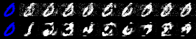
Reductions in \(\text{IP}^*\) are even more substantial and generally statistically significant, although the average degree of uncertainty is higher than for \(\text{IP}\): reductions range from around 25% (GMSC) to more than 90% (Circ). The only negative findings are for OL and MNIST, but they are insignificant. A qualitative inspection of the counterfactuals in Figure 5.2 suggests recognizable digits for the model trained with CT (bottom row), unlike the baseline (top row).
Actionability (RQ 5.2)
CT tends to improve actionability in the presence of immutable features, but this is not guaranteed if the assumptions in Proposition 5.1 are violated.
For synthetic datasets, we always protect the first feature; for all real-world tabular datasets we could identify and protect an age variable; for MNIST, we protect the five top and five bottom rows of pixels of the full image. Statistically significant reductions in costs overwhelmingly point in the positive direction reaching up to around 66% for GMSC data. Only in the case of Cred and MNIST, average costs increase, most likely because any benefits from protecting features are outweighed by an increase in costs required for greater plausibility. With respect to MNIST in particular, the weak baseline is susceptible to cheap adversarial attacks that significantly less costly to achieve that plausible counterfactuals. Finally, the findings for Adult are insignificant.
To further empirically evaluate the feature protection mechanism of CT beyond linear models covered in Proposition 5.1, we make use of integrated gradients (IG) (Sundararajan, Taly, and Yan 2017). IG calculates the contribution of each input feature towards a specific prediction by approximating the integral of the model output with respect to its input, using a set of samples that linearly interpolate between a test instance and some baseline instance. This process produces a vector of real numbers, one per input feature, which informs about the contribution of each feature to the prediction. The selection of an appropriate baseline is an important design decision (Sundararajan, Taly, and Yan 2017); to remain consistent in our evaluations, we use a baseline drawn at random from the uniform distribution \(\mathcal{U}(-1,1)\) for all datasets, which aligns with standard evaluation practices for IG. As the outputs are not bounded (i.e., they are real numbers), we standardize the integrated gradients across features to allow for a meaningful comparison of the results for different models.
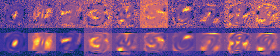
Qualitatively, the class-conditional integrated gradients in Figure 5.3 suggest that CT has the expected effect even for non-linear models: the model trained with CT (bottom row) is less sensitive (blue) to the five top and five bottom rows of pixels that were protected. Quantitatively, we observe substantial improvements for seven out of nine datasets, and inconclusive results for the remaining two datasets. Table 5.2 shows the average sensitivity to protected features measured by standardized integrated gradients for CT and BL along with 95% bootstrap confidence intervals: for the synthetic datasets, we observe strong reductions in sensitivity to the protected features for LS, OL and OL, in line with expectations. For the Moon dataset, the effect of feature protection is less pronounced but still in the expected direction. We also observe that confidence intervals are in some cases much tighter for models trained with CT: less noisy estimates for integrated gradients likely indicate that the model is more regularized and can be expected to behave more consistently across samples.
For real-world datasets, the sensitivity to the protected age variable is reduced by approximately a third for Adult, 20% for CH, and more than half for protected pixels in MNIST, mirroring the qualitative findings in Figure 5.3. In case of Cred, CT fully prevents the model from considering age as a factor in classification, with sensitivity reduced to zero. Only for GMSC, we observe negative impacts of CT, which we believe is due to any or all of the following: a) data assumptions are violated; b) the impact of other components of the CT objective outweighs expected effects of feature protection; or c) the baseline choice applied consistently to all datasets is not appropriate for GMSC.
5.4.3 Predictive Performance
Adversarial Robustness (RQ 5.3)
Models trained with CT are much more robust to gradient-based adversarial attacks than conventionally-trained (weak) baselines.
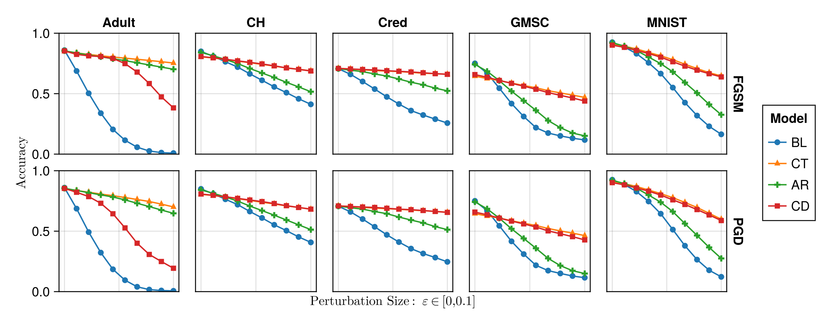
Test accuracies on clean and adversarially perturbed test data are shown in Figure 5.4. The perturbation size, \(\varepsilon\in[0,0.1]\), increases along the horizontal axis, where the case of \(\varepsilon=0\) corresponds to standard test accuracy for non-perturbed data. For synthetic datasets, predictive performance is virtually unaffected by perturbations for all models; those results are therefore omitted from Figure 5.4 in favor of better illustrations for the real-world data.
Focusing on the curves for CT and BL in Figure 5.4 for the moment,3 we find that standard test accuracy (\(\varepsilon=0\)) is largely unaffected by CT, while robustness against both types of attacks—FGSM (top row) and PGD (bottom row)—is greatly improved: while in some cases robust accuracies for the weak baseline drop to virtually zero (worse than random guessing) for large enough perturbation sizes, accuracies of CT models remain remarkably robust, even though robustness is not the primary objective of counterfactual training. In the only case where standard accuracy on unperturbed test data is substantially reduced for CT (GSMC), we note that robust accuracy decreases particularly fast for the weak baseline as the perturbation size increases. This seems to indicate that the standard accuracy for the weak baseline is inflated by sensitivity to meaningless associations in the data.
We also look at the validity of generated counterfactuals, or the proportion of counterfactuals that attain the target class, as presented in Table 5.3. We find that in many cases CT leads to substantial reductions in average validity, but this effect does not seem to be strongly influenced by the imposed mutability constraints (columns 1-2 vs columns 3-4). This result does not surprise us: by design, CT shrinks the solution space for valid counterfactual explanations, thus making it “harder” (and yet not “more costly”) to reach validity compared to the baseline model. As further discussed in the supplementary appendix, this should not be seen as a shortcoming of the method for a number of reasons: validity rates can be increased with longer searches; costs of found solutions still generally decrease, as we observe in our experiments; and achieving high validity does not entail that explanations are practical for the recipients (e.g., valid solutions may still be extremely costly) (Venkatasubramanian and Alfano 2020).
lSSSS Data & CT mut. & BL mut. & CT constr. & BL constr.
LS & 1.0 & 1.0 & 1.0 & 1.0
Circ & 1.0 & 0.51 & 0.71 & 0.48
Moon & 1.0 & 1.0 & 1.0 & 0.98
OL & 0.86 & 0.98 & 0.34 & 0.56
Adult & 0.68 & 0.99 & 0.7 & 0.99
CH & 1.0 & 1.0 & 1.0 & 1.0
Cred & 0.72 & 1.0 & 0.74 & 1.0
GMSC & 0.94 & 1.0 & 0.97 & 1.0
MNIST & 1.0 & 1.0 & 1.0 & 1.0
Avg. & 0.91 & 0.94 & 0.83 & 0.89
5.4.4 Ablation and Hyperparameter Settings
In this subsection, we use ablation studies to investigate how the different components of the counterfactual training objective in Equation 5.2 affect outcomes. Beyond this, we are also interested in understanding how CT depends on various other hyperparameters. To this end, we present the results from extensive grid searches run across all synthetic datasets.
Ablation (RQ 5.4)
All components of the CT objective affect outcomes, even independently, but the full objective achieves the most consistent improvements wrt. our goals.
We ablate the effect of both (1) the contrastive divergence component and (2) the adversarial loss included in the full CT objective in Equation 5.2. In the following, we refer to the resulting partial objectives as adversarial robustness (AR) and contrastive divergence (CD), respectively. We note that AR corresponds to a form of adversarial training and the CD objective is similar to that of a joint energy-based model. Therefore, the ablation also serves as a comparison of counterfactual training to stronger baselines, although we emphasize again that we do not seek to outperform SOTA methods in the domains of generative or robust machine learning, focusing CT squarely on models with high explainability and actionability in the context of algorithmic recourse.
Firstly, we find that both components play an important role in shaping final outcomes. Both AR and CD can independently improve the plausibility and adversarial robustness of models.
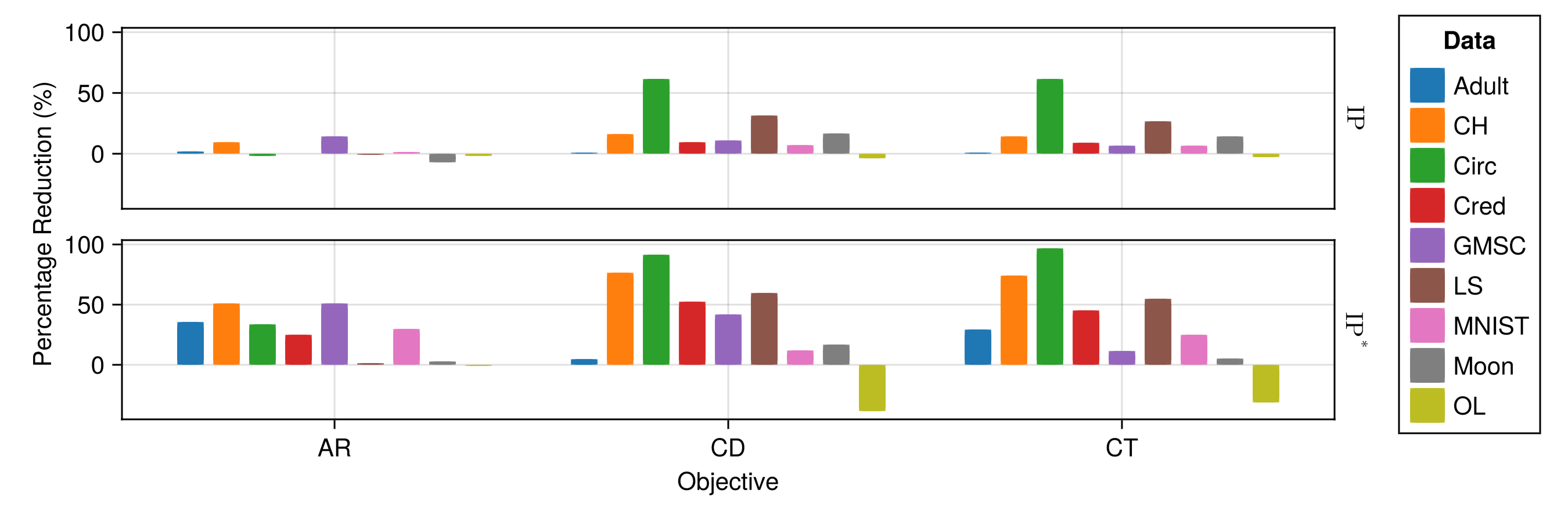
Concerning plausibility, Figure 5.5 shows the percentage reductions in implausibility for the partial and full objectives compared to the weak baseline. The results for \(\text{IP}\) and \(\text{IP}^*\) are shown in the top and bottom graphs, respectively, and the datasets are differentiated by color. We find that in the best identified hyperparameter settings, results for the full objective are predominantly affected by the contrastive divergence component, but the inclusion of adversarial loss leads to additional improvements for some datasets (Adult, MNIST). We penalize contrastive divergence twice as strongly as adversarial loss, which may explain why the former dominates. The outcome for Adult, in particular, demonstrates the benefit of including both components: as noted earlier, the large proportion of categorical features in this dataset seems to inhibit the generation of valid counterfactuals, which in turn appears to diminish the effect of the contrastive divergence component.
Looking at AR alone, we find that it produces mixed results for \(\text{IP}\), with strong positive results nonetheless dominating overall, reflecting previous findings from the related literature. In particular, for real-world tabular datasets, adversarial robustness seems to substantially benefit plausibility. In these cases, the inclusion of the AR component in the full objective also helps to substantially improve outcomes in relation to the partial CD objective: improvements in plausibility for the Adult and MNIST datasets are notably higher for full CT. In some cases—most notably GMSC and Cred—the full CT objective does not outperform the partial objectives, but still achieves the highest levels of adversarial robustness (Figure 5.4).
Zooming in on adversarial robustness, we find that the full CT objective consistently outperforms the partial objectives, which individually yield improvements. Consistent with the existing literature on JEMs (Grathwohl et al. 2020), CD yields substantially more robust models than the weak baseline at varying perturbation sizes (Figure 5.4). Similarly, AR yields consistent improvements in robustness, as expected. Still, we observe that in cases where either CD or AR show signs of degrading robust accuracy at higher perturbation sizes, the full CT objective maintains robustness. Much like in the context of plausibility, CT benefits from both components, highlighting the effectiveness of our approach to reusing nascent counterfactuals as AEs.
In summary, we find that the full CT objective strikes a balance between both components, thereby leading to the most consistent improvements with respect to plausibility and adversarial robustness.
Hyperparameter settings (RQ 5.5)
CT is quite sensitive to the choice of a CE generator and its hyperparameters but (1) we observe manageable patterns, and (2) we can usually identify settings that improve either plausibility or actionability, and typically both of them at the same time.
We evaluate the impacts of three types of hyperparameters on CT. In the following, we focus on the highlights and make the full results available in the supplementary appendix.
Firstly, we find that optimal results are generally obtained when using ECCCo to generate counterfactuals. Conversely, using a generator that may inhibit faithfulness (REVISE), regularly yields smaller improvements in plausibility and is more likely to even increase implausibility. The results of the grid search for REVISE also exhibit higher variability than the results for ECCCo and Generic. As argued above, this finding confirms our intuition that maximally faithful explanations are most suitable for counterfactual training.
Concerning hyperparameters that guide the gradient-based counterfactual search, we find that increasing \(T\), the maximum number of steps, generally yields better outcomes because more CEs can mature. Relatedly, we also find that the effectiveness and stability of CT is positively associated with the total number of counterfactuals generated during each training epoch. The impact of \(\tau\), the decision threshold, is more difficult to predict. On “harder” datasets it may be difficult to satisfy high \(\tau\) for any given sample (i.e., also factuals) and so increasing this threshold does not seem to correlate with better outcomes. In fact, \(\tau=0.5\) generally leads to optimal results as it is associated with high proportions of mature counterfactuals. This is likely because the special case of \(\tau=0.5\) corresponds to equal class probabilities, so a counterfactual is considered mature when the logit for the target class is higher than the logits for all other classes.
Secondly, the strength of the energy regularization, \(\lambda_{\text{reg}}\), is highly impactful and should be set sufficiently high to avoid common problems associated with exploding gradients. The sensitivity with respect to \(\lambda_{\text{div}}\) and \(\lambda_{\text{adv}}\) is much less evident. While high values of \(\lambda_{\text{reg}}\) may increase the variability in outcomes when combined with high values of \(\lambda_{\text{div}}\) or \(\lambda_{\text{adv}}\), this effect is not particularly pronounced. These results mirror our observations from the ablation studies and lend further weight to the argument that CT benefits from both components.
Finally, we also observe desired improvements when CT was combined with conventional training and employed only for the final 50% of epochs of the complete training process. Put differently, CT can improve the explainability of models in a post-hoc, fine-tuning manner.
5.5 Discussion
As our results indicate, counterfactual training achieves its objective of producing models that are more explainable. Nonetheless, these advantages come with certain limitations.
Immutable features may have proxies. We propose a method to modify the sensitivity of a model to certain features, and thus increase the actionability of the generated CEs. However, it requires that model owners define the mutability constraints for (all) features considered by the model. Even if all immutable features are protected, there may exist proxies that are theoretically mutable (and hence should not be protected) but preserve enough information about the principals to hinder these protections. Delineating actionability is a major open challenge in the AR literature (see, e.g., (Venkatasubramanian and Alfano 2020)) impacting the capacity of CT to fulfill its intended goal.
Interventions on features may have implications for fairness. Modifying the sensitivity of a model to certain features may also have implications for the fair and equitable treatment of decision subjects. Model owners could misuse this solution by enforcing explanations based on features that are more difficult to modify by some (group of) decision subjects. For example, consider the Adult dataset used in our experiments, where workclass or education may be more difficult to change for underprivileged groups. When applied irresponsibly, CT could result in an unfairly assigned burden of recourse (Sharma, Henderson, and Ghosh 2020), threatening the equality of opportunity in the system (Bell et al. 2024). Nonetheless, these phenomena are not specific to CT.
Plausibility is costly. As noted before, more plausible counterfactuals are inevitably more costly (Altmeyer et al. 2024). CT improves plausibility and robustness, but this can negatively affect average costs and validity whenever cheap, implausible, and adversarial explanations are removed from the solution space.
CT increases training times. Just like contrastive and robust learning, CT is more resource-intensive than conventional regimes. Three factors mitigate this effect: (1) CT yields itself to parallel execution; (2) it amortizes the cost of CEs for the training samples; and (3) our preliminary findings suggest that it can be used to fine-tune conventionally-trained models.
We also highlight three key directions for future research. Firstly, it is an interesting challenge to extend CT beyond classification settings. Our formulation relies on the distinction between target and non-target classes, requiring the output space to be discrete. Thus, it does not apply to ML tasks where the change in outcome cannot be readily discretized. Classification remains the focus of CE and algorithmic recourse research; other settings have attracted some interest (e.g., regression (Spooner et al. 2021)), but there is little consensus on how to extend the notion of CEs.
Secondly, our analysis covers CE generators with different characteristics, but it is interesting to extend it to more algorithms, including ones that do not rely on computationally costly gradient-based optimization. This should reduce training costs while possibly preserving the benefits of CT.
Finally, we believe that it is possible to considerably improve hyperparameter selection procedures. Our method benefits from the tuning of certain key hyperparameters but we have relied exclusively on grid searches. Future work on CT could benefit from more sophisticated approaches. Notably, CT is iterative, which makes methods such as Bayesian or gradient-based optimization applicable (see, e.g., (Bischl et al. 2023)).
5.6 Conclusion
State-of-the-art machine learning models are prone to learning complex representations that cannot be interpreted by humans. Existing work on counterfactual explanations has largely focused on designing tools to generate plausible and actionable explanations for any model. In this work, we instead hold models accountable for delivering such explanations. We introduce counterfactual training: a novel training regime that integrates recent advances in contrastive learning, adversarial robustness, and CE to incentivize highly explainable models. Through theoretical results and extensive experiments, we demonstrate that CT satisfies this goal while promoting adversarial robustness of models. Explanations generated from CT-based models are both more plausible (compliant with the underlying data-generating process) and more actionable (compliant with user-specified mutability constraints), and thus meaningful to recipients. In turn, our work highlights the value of simultaneously improving models and their explanations.
5.7 Acknowledgments
Some of the authors were partially funded by ICAI AI for Fintech Research, an ING—TU Delft collaboration. Research reported in this work was partially facilitated by computational resources and support of the DelftBlue high-performance computing cluster at TU Delft ((DHPC) 2022).
During initial prototyping of CT we also tested an implementation that relies on generating counterfactuals and adversarial examples at the batch level with no discernible difference in outcomes, but increased training times.↩︎
https://github.com/JuliaTrustworthyAI/CounterfactualTraining.jl↩︎
The results for AR and CD are discussed in the context of ablation below.↩︎