Appendix G — Supplementary Material for Chapter 6
Artificial Intelligence, Trustworthy AI, Counterfactual Explanations, Algorithmic Recourse
In this section, we present additional experimental results that we did not include in the body of the paper for the sake of brevity. We still choose to provide them as additional substantiation of our arguments here. This section also contains additional details concerning the experiment setup for our examples where applicable.
G.1 Are Neural Networks Born with World Maps?
The initial feature matrix \(X^{(n \times m)}\) is made up of \(n=4,217\) and \(m=10\) features. We add a total of \(490\) random features to \(X\) to simulate the fact that not all features ingested by Llama-2 are necessarily correlated with geographical coordinates. That yields \(500\) features in total. The training subset contains \(3,374\) randomly drawn samples, while the remaining \(843\) are held out for testing. The single hidden layer of the untrained neural network has \(400\) neurons.
G.2 Autoencoders as Economic Growth Predictors
This is an additional example that we have not discuss in the body of the paper. Here, we build forth on an application in Economics. However, we now seek to not only predict economic growth from the yield curve, but also extract meaningful features for downstream inference tasks. For this, we will use a neural network architecture.
G.2.1 Data
To estimate economic growth, we will rely on a quarterly series of the real gross domestic product (GDP) provided by the Federal Reserve Bank of St. Louis. The data arrives in terms of levels of real GDP. In order to estimate growth, we transform the data using log differences. Since our yield curve data is daily, we aggregate it to the quarterly frequency by taking averages of daily yields for each maturity. We also standardize yields since deep learning models tend to perform better with standardized data (Michal S Gal 2019). Since COVID-19 was a substantial structural break in the time series, we also filter out all observations after 2018.
G.2.2 Model
Using a simple autoencoder architecture, we let our model \(g_t\) denote growth and our conditional \(\mathbf{r}_t\) the matrix of aggregated Treasury yield rates at time \(t\). Finally, we let \(\theta\) denote our model parameters. Formally, we are interested in maximizing the likelihood \(p_{\theta}(g_t|\mathbf{r}_t)\).
The encoder consists of a single fully connected hidden layer with 32 neurons and a hyperbolic tangent activation function. The bottleneck layer connecting the encoder to the decoder, is a fully connected layer with 6 neurons. The decoder consists of two fully connected layers, each with a hyperbolic tangent activation function: the first layer consists of 32 neurons and the second layer will have the same dimension as the input data. The output layer consists of a single neuron for our output variable, \(g_t\). We train the model over 1,000 epochs to minimize mean squared error loss using the Adam optimizer (Kingma and Ba 2017).
The in-sample fit of the model is shown in the left chart of Figure G.1, which shows actual GDP growth and fitted values from the autoencoder model. The model has a large number of free parameters and captures the relationship between economic growth and the yield curve reasonably well, as expected. Since our primary goal is not out-of-sample prediction accuracy but feature extraction for inference, we use all of the available data instead of reserving a hold-out set. As discussed above, we also know that the relationship between economic growth and the yield curve is characterized by two main factors: the level and the spread. Since the model itself is fully characterized by its parameters, we would expect that these two important factors are reflected somewhere in the latent parameter space.
G.2.3 Linear Probe
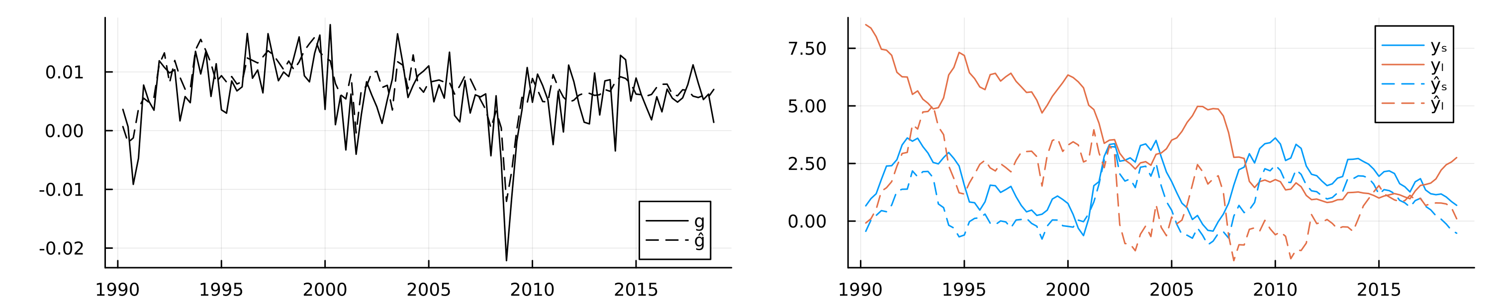
While the loss function applies most direct pressure on layers near the final output layer, any information useful for the downstream task first needs to pass through the bottleneck layer (Alain and Bengio 2016). On a per-neuron basis, the pressure to distill useful representation is therefore likely maximized there. Consequently, the bottleneck layer activations seem like a natural place to start looking for compact, meaningful representations of distilled information. We compute and extract these activations \(A_t\) for all time periods \(t=1,...,T\). Next, we use a linear probe to regress the observed yield curve factors on the latent embeddings. Let \(Y_t\) denote the vector containing the two factors of interest in time \(t\): \(y_{t,l}\) and \(y_{t,s}\) for the level and spread, respectively. Formally, we are interested in the following regression model: \(p_{w}(Y_t|A_t)\) where \(w\) denotes the regression parameters. We use Ridge regression with \(\lambda\) set to \(0.1\). Using the estimated regression parameters \(\hat{w}\), we then predict the yield curve factors : \(\hat{Y}_t=\hat{w}^{\prime}A_t\).
The in-sample predictions of the probe are shown in the right chart of Figure G.1. Solid lines show the observed yield curve factors over time, while dashed lines show predicted values. We find that the latent embeddings predict the two yield curve factors reasonably well, in particular the spread.
Did the neural network now learn an intrinsic understanding of the economic relationship between growth and the yield curve? To us, that would be too big of a statement. Still, the current form of information distillation can be useful, even beyond its intended use for monitoring models. For example, an interesting idea could be to use the latent embeddings as features in a more traditional and interpretable econometric model. To demonstrate this, let us consider a simple linear regression model for GDP growth. We might be interested in understanding to what degree economic growth in the past is associated with economic growth today. As we might expect, linearly regressing economic growth on lagged growth, as in column (1) of Table G.1, yields a statistically significant coefficient. However, this coefficient suffers from confounding bias since there are many other confounding variables at play, of which some may be readily observable and measurable, but others may not.
We e.g. already mentioned the relationship between interest rates and economic growth. To account for that, while keeping our regression model as parsimonious as possible, we could include the level and the spread of the US Treasury yield curve as additional regressors. While this slightly changes the estimated magnitude of the coefficient on lagged growth, the coefficients on the observed level and spread are statistically insignificant (column (2) in Table G.1). This indicates that these measures may be too crude to capture valuable information about the relationship between yields and economic growth. Because we have included two additional regressors with little to no predictive power, the model fit as measured by the Bayes Information Criterium (BIC) has actually deteriorated.
Column (3) of Table G.1 shows the effect of instead including one of the latent embeddings that we recovered above in the regression model. In particular, we pick the one latent embedding that we have found to exhibit the most significant effect on the output variable in a separate regression of growth on all latent embeddings. The estimated coefficient on this latent factor is small in magnitude, but statistically significant. The overall model fit, as measured by the BIC has improved and the magnitude of the coefficient on lagged growth has changed quite a bit. While this is still a very incomplete toy model of economic growth, it appears that the compact latent representation we recovered can be used in order to mitigate confounding bias.
| GDP Growth | |||
| (1) | (2) | (3) | |
| (Intercept) | 0.004*** | 0.002 | 0.004*** |
| (0.001) | (0.002) | (0.001) | |
| Lagged Growth | 0.398*** | 0.385*** | 0.344*** |
| (0.087) | (0.089) | (0.088) | |
| Spread | 0.000 | ||
| (0.001) | |||
| Level | 0.000 | ||
| (0.000) | |||
| Embedding 6 | 0.008* | ||
| (0.003) | |||
| Obs. | 114 | 114 | 114 |
| BIC | -860.391 | -857.429 | -864.499 |
| R² | 0.158 | 0.168 | 0.203 |
G.3 LLMs for Economic Sentiment Prediction
G.3.1 Linear Probes
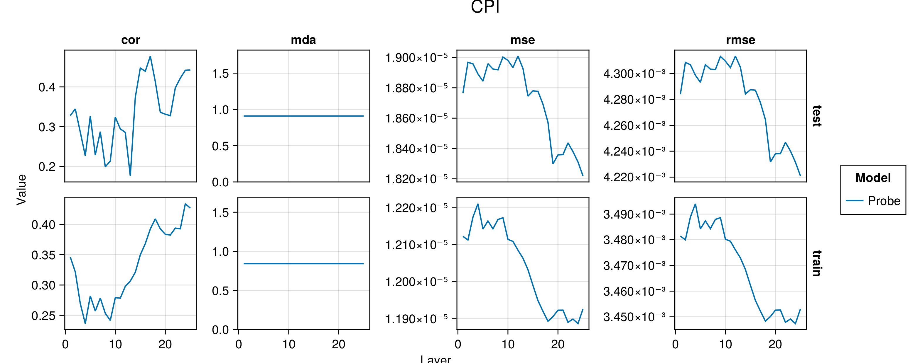
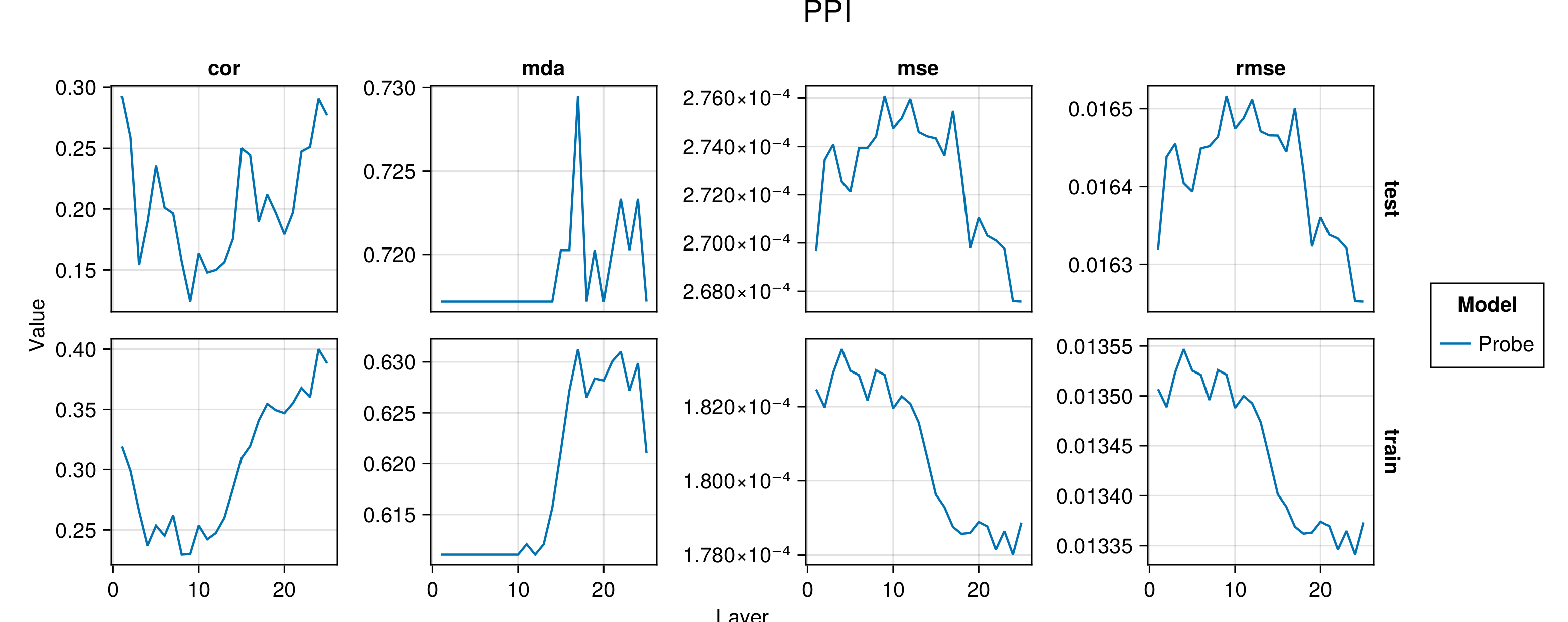
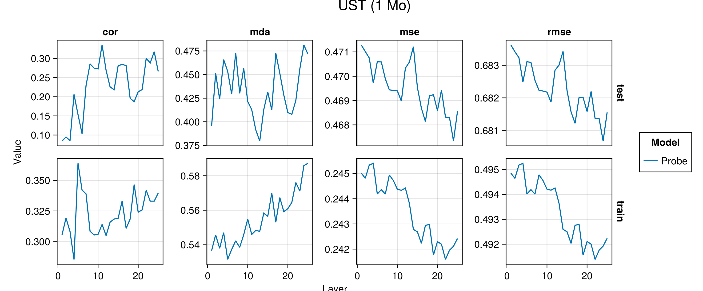
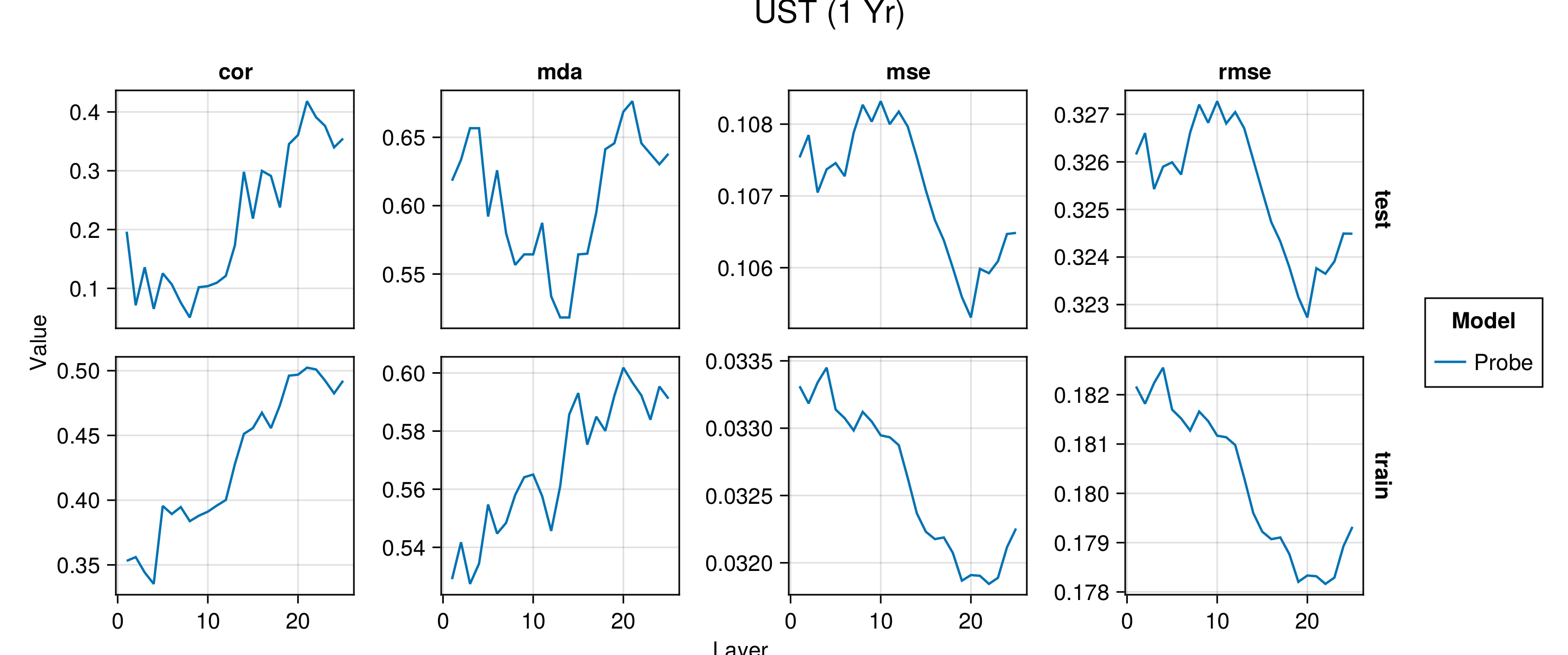
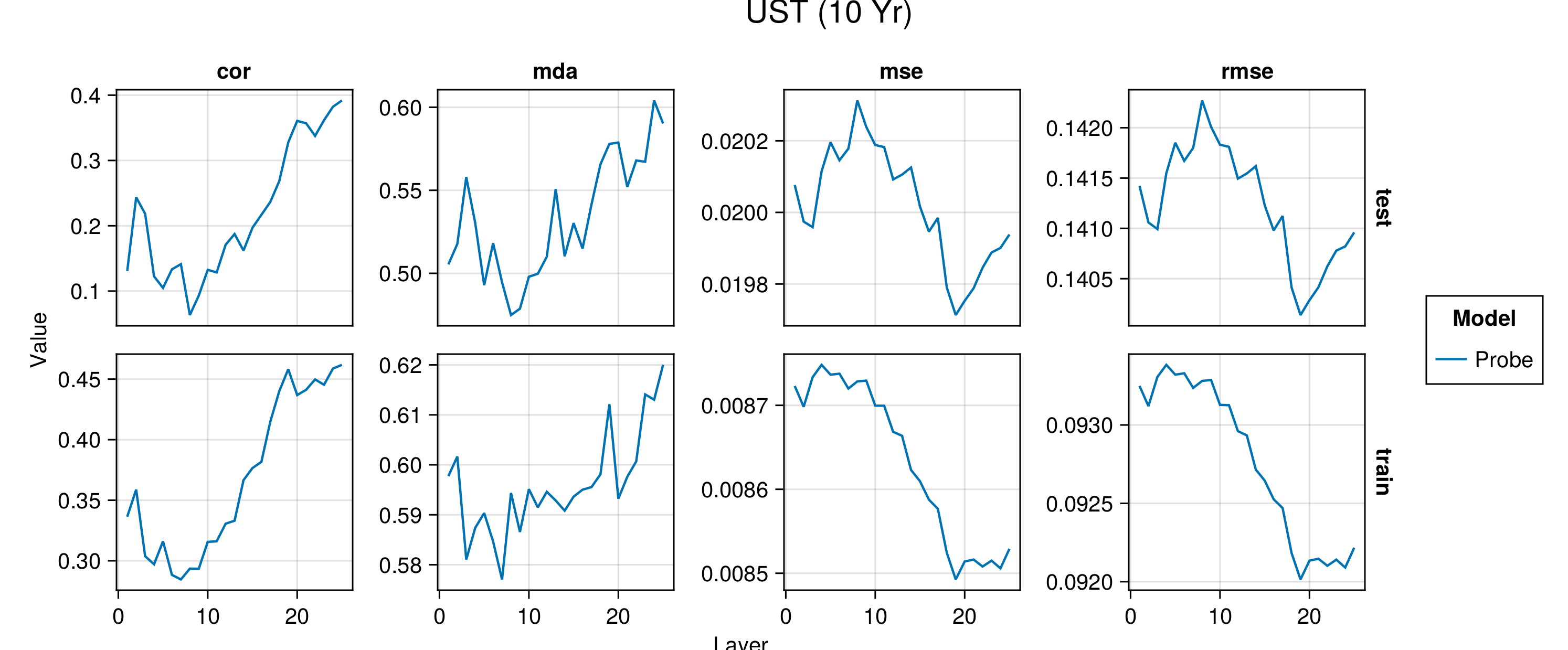
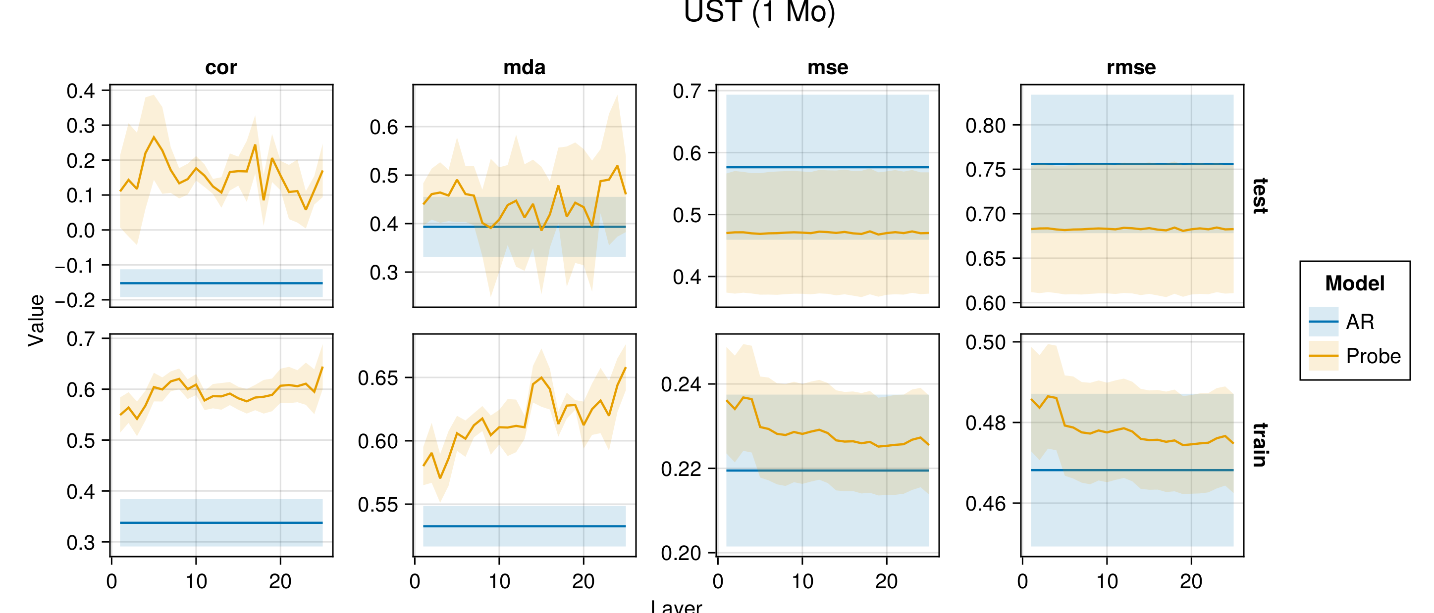
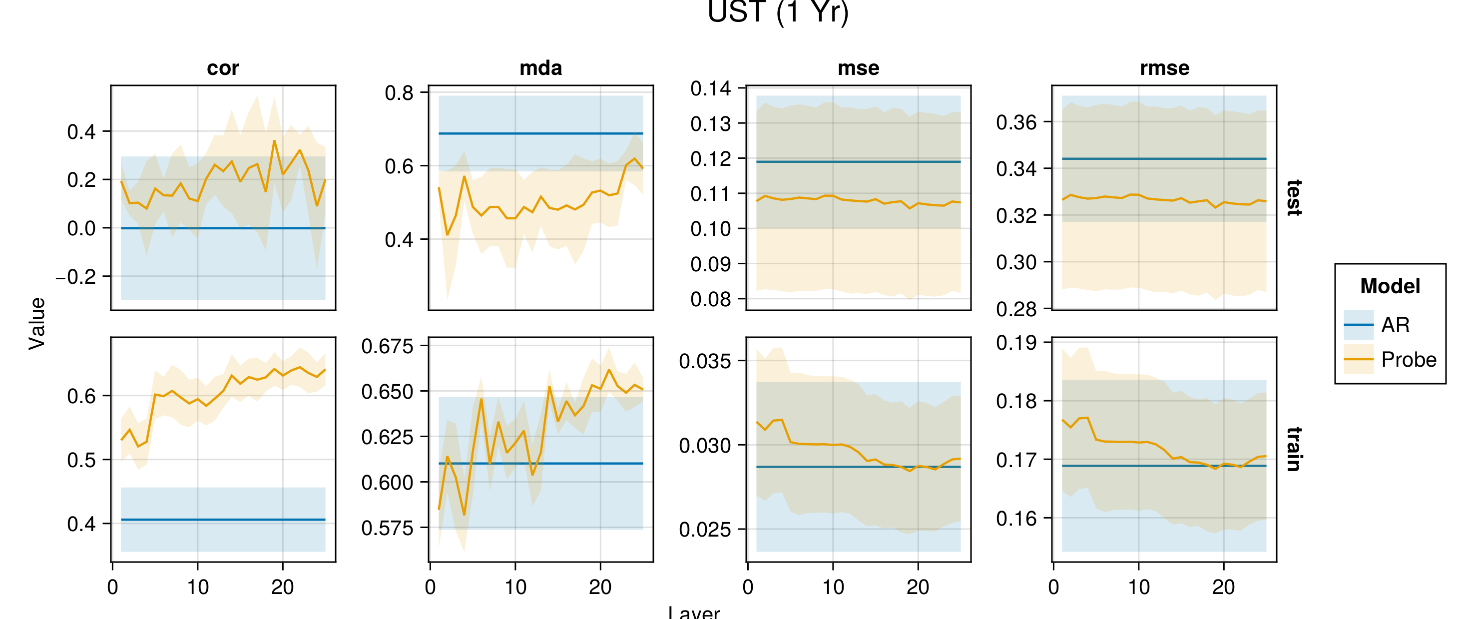
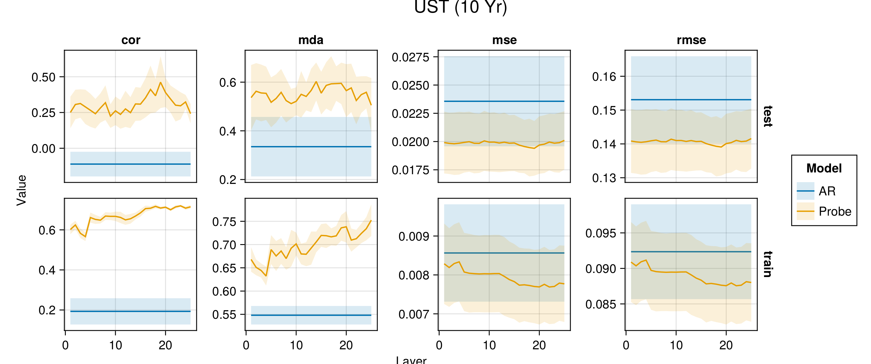
Figure G.2 to Figure G.6 present average performance measures across folds for all indicators each time for the train and test set. We report the correlation between predictions and observed values (‘cor’), the mean directional accuracy (‘mda’), the mean squared error (‘mse’) and the root mean squared error (‘rmse’). The model depth—as indicated by the number of the layer—increases along the horizontal axis.
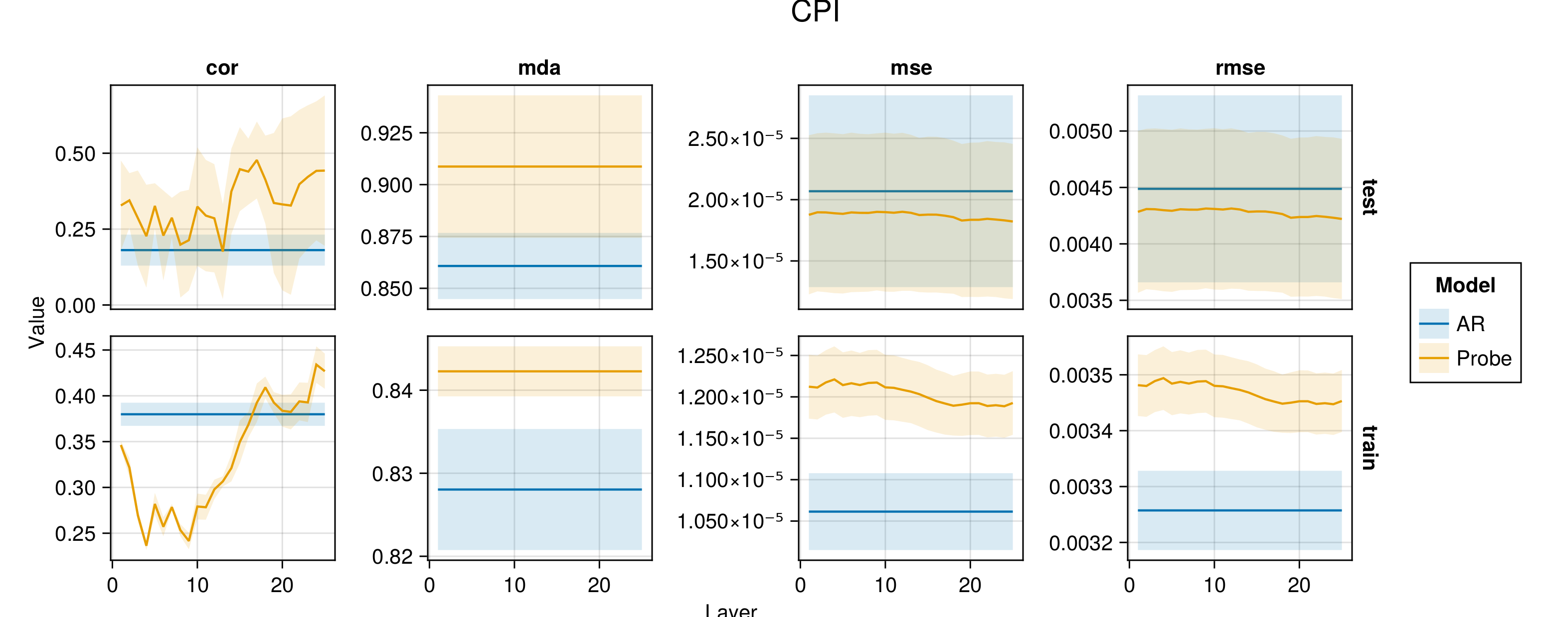
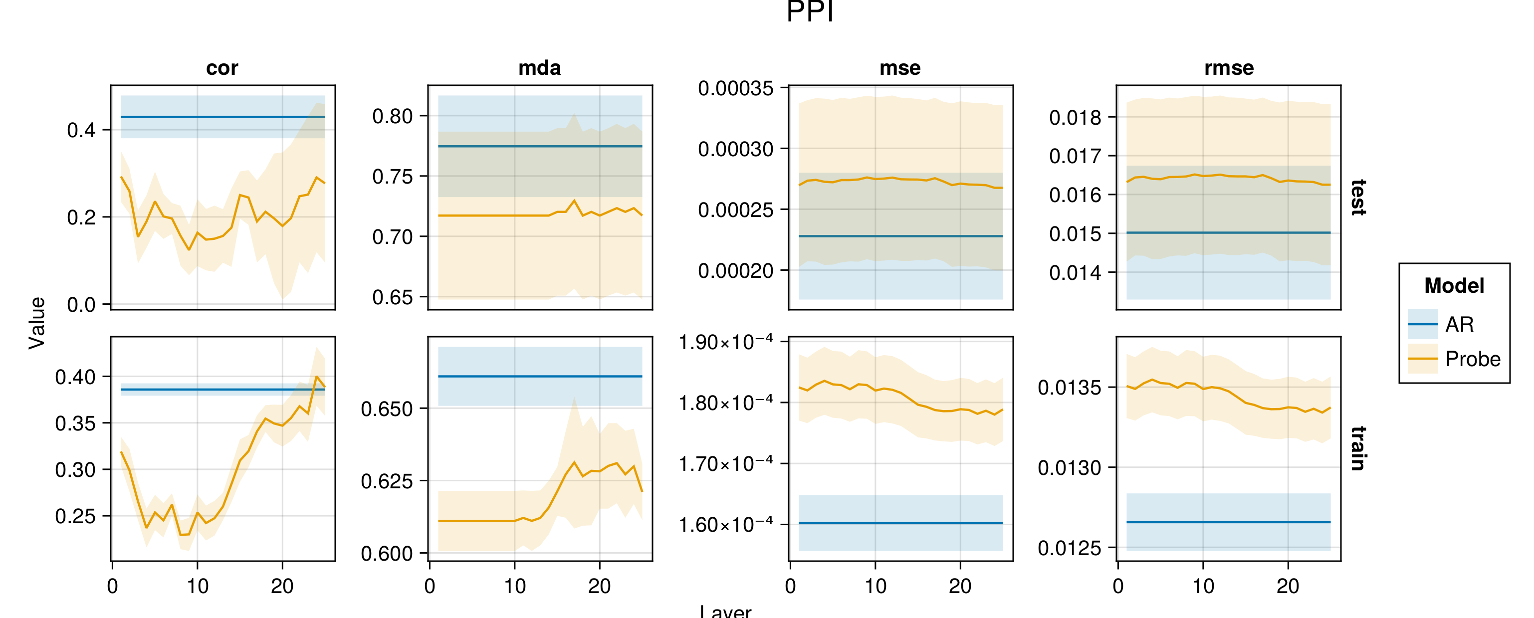
Figure G.7 to Figure G.11 present the same performance measures, also for the baseline autoregressive model. Shaded areas show the variation across folds.
G.3.2 Spark of Econonomic Understanding?
Below we present the 10 sentences in each category that were used to generate the probe predictions plotted in Figure 6.4. In each case, the first 5 sentences were composed by ourselves. The following 5 sentences were generated using ChatGPT 3.5 using the following prompt followed by the examples in each category:
“I will share 5 example sentences below that sound a bit like they are about price deflation but are really about a deflation in the numbers of doves. Please generate an additional 25 sentences that are similar. Concatenate those sentences to the example string below, each time separating a sentence using a semicolon (just follow the same format I’ve used for the examples below). Please return only the concatenated sentences, including the original 5 examples.
Here are the examples:”
This was followed up with the following prompt to generate additional sentences:
“Please generate X more sentences in the same manner and once again return them in the same format. Do not recycle sentences you have already generated, please.”
All of the sentences were then passed through the linear probe for the CPI and sorted in ascending or descending order depending on the context (inflation or deflation). We then carefully inspected the list of sentences and manually selected 5 additional sentences to concatenate to the 5 sentences we composed ourselves.
G.3.2.1 Inflation/Prices
The following sentences were used:
Consumer prices are at all-time highs.;Inflation is expected to rise further.;The Fed is expected to raise interest rates to curb inflation.;Excessively loose monetary policy is the cause of the inflation.;It is essential to bring inflation back to target to avoid drifting into hyperinflation territory.;Inflation is becoming a global phenomenon, affecting economies across continents.;Inflation is reshaping the dynamics of international trade and competitiveness.;Inflationary woes are prompting governments to reassess fiscal policies and spending priorities.;Inflation is reshaping the landscape of economic indicators, challenging traditional forecasting models.;The technology sector is not immune to inflation, facing rising costs for materials and talent.
G.3.2.2 Inflation/Birds
The following sentences were used:
The number of hawks is at all-time highs.;Their levels are expected to rise further.;The Federal Association of Birds is expected to raise barriers of entry for hawks to bring their numbers back down to the target level.;Excessively loose migration policy for hawks is the likely cause of their numbers being so far above target.;It is essential to bring the number of hawks back to target to avoid drifting into hyper-hawk territory.;The unprecedented rise in hawk figures requires a multi-pronged approach to wildlife management.;Environmental agencies are grappling with the task of addressing the inflationary hawk numbers through targeted interventions.;The burgeoning hawk figures highlight the need for adaptive strategies to manage and maintain a healthy avian community.;The unprecedented spike in hawk counts highlights the need for adaptive and sustainable wildlife management practices.;Conservationists advocate for proactive measures to prevent further inflation in hawk numbers, safeguarding the delicate balance of the avian ecosystem.
G.3.2.3 Deflation/Prices
The following sentences were used:
Consumer prices are at all-time lows.;Inflation is expected to fall further.;The Fed is expected to lower interest rates to boost inflation.;Excessively tight monetary policy is the cause of deflationary pressures.;It is essential to bring inflation back to target to avoid drifting into deflation territory.;The risk of deflation may increase during periods of economic uncertainty.;Deflation can lead to a self-reinforcing cycle of falling prices and reduced economic activity.;The deflationary impact of reduced consumer spending can ripple through the entire economy.;Falling real estate prices can contribute to deflation by reducing household wealth and confidence.;The deflationary impact of falling commodity prices can have ripple effects throughout the global economy.
G.3.2.4 Deflation/Birds
The following sentences were used:
The number of doves is at all-time lows.;Their levels are expected to fall further.;The Federal Association of Birds is expected to lower barriers of entry for doves to bring their numbers back up to the target level.;Excessively tight migration policy for doves is the likely cause of their numbers being so far below target.;Dovelation risks loom large as the number of doves continues to dwindle.;The number of doves is experiencing a significant decrease in recent years.;It is essential to bring the numbers of doves back to target to avoid drifting into dovelation territory.;A comprehensive strategy is needed to reverse the current dove population decline.;Experts warn that without swift intervention, we may witness a sustained decrease in dove numbers.
We think that this sort of manual, LLM-aided adversarial attack against another LLM can potentially be scaled up to allow for rigorous testing, which we will turn to next.
G.4 Toward Parrot Tests
In our experiments from Section Section 6.3.3, we considered the following hypothesis tests as a minimum viable testing framework to assess if our probe results (may) provide evidence for an actual ‘understanding’ of key economic relationships learned purely from text:
Proposition G.1 (Parrot Test)
H0 (Null): The probe never predicts values that are statistically significantly different from \(\mathbb{E}[f(\varepsilon)]\).
H1 (Stochastic Parrots): The probe predicts values that are statistically significantly different from \(\mathbb{E}[f(\varepsilon)]\) for sentences related to the outcome of interest and those that are independent (i.e. sentences in all categories).
H2 (More than Mere Stochastic Parrots): The probe predicts values that are statistically significantly different from \(\mathbb{E} [f(\varepsilon)]\) for sentences that are related to the outcome variable (IP and DP), but not for sentences that are independent of the outcome (IB and DB).
To be clear, if in such a test we did find substantial evidence in favour of rejecting both HO and H1, this would not automatically imply that H2 is true. But to even continue investigating, if based on having learned meaningful representation the underlying LLM is more than just a parrot, it should be able to pass this simple test.
In this particular case, Figure 6.4 demonstrates that we find some evidence to reject H0 but not H1 for FOMC-RoBERTa. The median linear probe predictions for sentences about inflation and deflation are indeed substantially higher and lower, respectively than for random noise. Unfortunately, the same is true for sentences about the inflation and deflation in the number of birds, albeit to a somewhat lower degree. This finding holds for both inflation indicators and to a lesser degree also for yields at different maturities, at least qualitatively.
We should note that the number of sentences in each category is very small here (10), so the results in Figure 6.4 cannot be used to establish statistical significance. That being said, even a handful of convincing counter-examples should be enough for us to seriously question the claim, that results from linear probes provide evidence in favor of real ‘understanding’. In fact, even a handful of sentences for which any human annotator would easily arrive at the conclusion of independence, a prediction by the probe in either direction casts doubt.
G.5 Code
All of the experiments were conducted on a MacBook Pro, 14-inch, 2023, with an Apple M2 Pro chip and 16GB of RAM. Forward passes through the FOMC-RoBERTa were run in parallel on 6 threads. All our code will be made publicly available. For the time being, an anonymized version of our code repository can be found here: https://anonymous.4open.science/r/spurious_sentience/README.md.